Pneumonia Detection using Deep Learning

In this Python machine learning project, we will determine whether a person suffers from pneumonia or not, if yes, then determine whether it is caused by bacteria or viruses. This is a multi-classification problem. For this, we will build a model to detect if given x-ray images have pneumonia or not. We will convert all images of x-ray to number format using ‘OpenCV’ and then feed them into the Convolutional neural network which will help us to predict the output. Let’s start the Pneumonia Detection project using Deep Learning.

What is Pneumonia?

Pneumonia is a lung infection caused by bacteria, viruses, or fungal spores. This infection causes inflammation in the air sacs of the lungs, which are called alveoli. The alveoli gets clogged with fluid or pus, making breathing difficult. If not treated promptly, pneumonia can develop into a significant health problem or even be fatal.

What is a Convolutional Neural Network?

A convolutional neural network is a type of deep neural network, which is used for image processing and its classification. As the name suggests, Convolutional Network helps for classifying complex images by multiplying pixel value with weights and then summing them. Keras Api provides a Conv2D function in order to use a convolutional network layer. Let’s see some parameters of Conv2D function which we are going to use in this project

Input : This is the input shape dimension of our convolutional layer. It expects the shape of input images in rows(Image height), columns(Image width), and channels (depth) format.

Filter or Kernel : Filters detect spatial patterns such as edges in an image by detecting the changes in intensity values of the image resulting in a feature map. Size of filters are mostly three dimensional with the same number of channels but with fewer height and width.

Strides : The number of shifting between application of filter to the input image is called strides. So strides (1,1) means moving the filter one pixel right for each horizontal movement of the filter and one pixel down for each vertical movement of the filter when creating the feature map.

Padding : If our image array size is for example 8×8 and if we apply a filter of 3×3 then our resulting array size will be 6×6. So you can see there is loss in our array as 8×8 image size becomes 6×6 this is called a border effect problem. So to overcome this we will pad layers of 0’s in order to maintain the same size of the array throughout.

Prerequisites for this project:

You can install all the modules for this project using following command:

pip install numpy, opencv-python , tensorflow, sklearn

The versions which are used in this project for python and its corresponding modules are as follows:

1) python : 3.8.5
2) tensorflow : 2.3.1 *Note* : TensorFlow version should be 2.2 or higher in
order to use keras or else install keras directly
3) opencv : 4.1.2
4) sklearn : 0.24.2
5) numpy : 1.19.5

I am going to use Google’s Colab Platform for model training as it provides a free GPU utility.

Dataset for Pneumonia Detection Project

Please download the Dataset for pneumonia detection project from the following link: Pneumonia Detection Project Dataset

Download Pneumonia Detection Project Code

Please download the source code of pneumonia detection with deep learning: Pneumonia Detection Deep learning Project Code

Project Structure :

xray : This is the parent directory of our dataset.

train/normal : This directory contains normal x-ray images for training sets. Total number of images is 1,341.

train/pneumonia : This directory contains pneumonia x-ray images for training sets. Total number of images is 3,875.

test/normal : This directory contains normal x-ray images for testing sets. Total number of images is 234.
test/pneumonia : This directory contains pneumonia x-ray images for testing sets. Total number of images is 390.

pneumonia_detection.py : This is the file where we will write our code to train our model and for prediction.

s2s/ : This directory contains optimizer, metrics and the weights of our trained
model.

Steps for Deep Learning Pneumonia Detection Project:

1) Import all Libraries

Firstly we will create a file called ‘pneumonia_detection.py’ and import all the libraries which have been shared in the prerequisites section.

Code:

#ProjectGurukul
#load all required libraries
import cv2
import numpy as np
from sklearn.preprocessing import OneHotEncoder
from tensorflow.keras.models import load_model,Model
from tensorflow.keras.optimizers import Adam
from tensorflow.keras.layers import Dense,Input,Conv2D,Flatten,MaxPool2D
from tensorflow.keras.preprocessing.image import ImageDataGenerator
import glob

#import below library only if you are using google colab
#from google.colab.patches import cv2_imshow

2) Parse the Dataset file

The Structure of our Dataset is

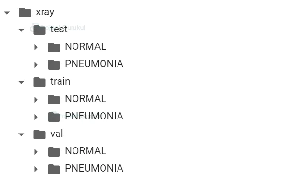
As you can see we have three folders ‘train’ , ‘test’ and ‘val’ in ‘xray’ which is the parent folder. This folder contains two subfolders i.e. ‘NORMAL’ and ‘PNEUMONIA’. ‘NORMAL’ folder contains normal x-ray(no pneumonia) images and the ‘PNEUMONIA’ folder contains pneumonia x-ray (has pneumonia) images. We will take help from the ‘train’ folder to train our model and ‘test’ folder to test our trained model.

Code:

#train and test directory path
train_dir= "xray/train/"
test_dir= "xray/test/"
im_size= 200
batch_size= 32

We will create a function ‘dir_img_lab()’ which takes parameters as ‘train’ or ‘test’ directory. With the help of this it will store normal and pneumonia x-ray images of a given directory as input. Along with this, it will also store labels of respective images. Labels for normal x-rays will be ‘normal’ and for pneumonia x-rays will be ‘bacteria’ and ‘virus’. With the help of the ‘glob’ module we will retrieve files matching a specified pattern.

Code:

def dir_img_lab(dir):
#fetch all the normal xray images and labels from given directory
norm_img = glob.glob(dir+"NORMAL/*.jpeg")
norm_labels = np.array(['normal']*len(norm_img))

#fetch all the pneumonia xray images and labels from given directory
pnm_img = glob.glob(dir+"PNEUMONIA/*.jpeg")
pnm_labels = np.array(list(map(lambda x: x.split("_")[1],pnm_img)))

return norm_img,norm_labels,pnm_img,pnm_labels

#get the normal and pneumonia images for training and testing
#and also get the labels
trn_norm_img,trn_norm_lab,trn_pnm_img,trn_pnm_lab= dir_img_lab(train_dir)
tst_norm_img,tst_norm_lab,tst_pnm_img,tst_pnm_lab= dir_img_lab(test_dir)

After completing the second step, we will get four datas for training i.e. train normal images, train normal labels, train pneumonia images, train pneumonia labels and the same for testing data also.

3) Image Processing

With the help of ‘opencv’ library we will read our images in a grayscale format (monochromatic shades of black to white) using the ‘imread()’ function. Grayscale images have only one channel (matrix) and its pixel (every element) value shows intensity, which varies between 0 (black) to 255 (white). All images in our dataset are in different shapes, so resize all images to the same width and height i.e. in our case 200×200. After resizing all images, we will reshape them to make our array of rank 4 i.e. after reshaping our array will have ( Image Index , Image Height , Image width , Image depth ). Depth will be 1 as Grayscale has only one channel.

Code:

def get_x(files):
#create a numpy array of the shape
#(number of images, image size , image size, 1 for grayscale channel ayer)
#this will be input for model
train_x = np.zeros((len(files), im_size, im_size,1), dtype='float32')

#iterate over img_file of given path
for i, img_file in enumerate(files):
#read the image file in a grayscale format and convert into numeric format
#resize all images to one dimension i.e. 200x200
img = cv2.resize(cv2.imread(img_file,cv2.IMREAD_GRAYSCALE),((im_size,im_size)))
#reshape array to the train_x shape
#1 for grayscale format
img_array = np.expand_dims(np.array(img[...,::-1].astype(np.float32)).copy(), axis=0)
train_x[i] = img_array.reshape(img_array.shape[1],img_array.shape[2],1)

return train_x

#pass the normal and pneumonia images of training and testing sets
trn_norm_x= get_x(trn_norm_img)
trn_pnm_x= get_x(trn_pnm_img)
tst_norm_x= get_x(tst_norm_img)
tst_pnm_x= get_x(tst_pnm_img)

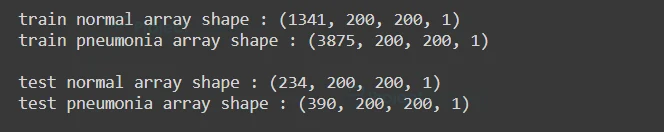
We can see the shape of our training and testing image data array

Code:

print("train normal array shape :",trn_norm_x.shape)
print("train pneumonia array shape :",trn_pnm_x.shape)
print("\ntest normal array shape :",tst_norm_x.shape)
print("test pneumonia array shape :",tst_pnm_x.shape)

Output:

4) Training and Testing Sets

Use the output of the third step to make training and testing sets. We will take help of numpy’s append function to append two arrays i.e. add a second array to the end of the first array along axis 0. So in our case we will append a pneumonia array with a normal array. Do the same process for normal labels and pneumonia labels.

Code:

#append pneumonia array to normal array and
#append pneumonia labels to normal labels of training
x_train = np.append(trn_norm_x,trn_pnm_x,axis=0)
y_train = np.append(trn_norm_lab,trn_pnm_lab)

#above process for testing as well
x_test = np.append(tst_norm_x,tst_pnm_x,axis=0)
y_test = np.append(tst_norm_lab,tst_pnm_lab)

As we know our label contains datas like ‘normal’ for normal data and ‘bacteria’ , ‘virus’ for pneumonia data, which is in text format. We will need to convert them into numeric format for our model. So we will be using the ‘OneHotEncoder()’ function. One-hot encoding deals the data in binary format so we encode the categorical data to binary format. One-hot means that we can only make a value 1(true) if it is present in the vector or else 0(false). So every data has its unique representation in vector format.

Code:

#This will be the target for the model.
#convert labels into numerical format
encoder = OneHotEncoder(sparse=False)
y_train_enc= encoder.fit_transform(y_train.reshape(-1,1))
y_test_enc= encoder.fit_transform(y_test.reshape(-1,1))

5) Data Augmentation

Augmentation is basically a technique which can be used to artificially expand the size of images in real time by creating various modified versions. This will help the model to generalize and also it will improve performance.

Some of the most used Augmentation techniques for images are :

• Position Augmentation : Changes the position of pixels (elements in our matrix) by using Scaling, Translation, Rotation, Flipping and Cropping techniques.
• Color Augmentation : Changes the value of pixels(elements in our matrix) by changing the Brightness, Contrast, Hue and Saturation levels.

We will take the help of ‘ImageDataGenerator()’ to create different types of training and testing image arrays by modifying the original array data.

Code:

#Image augmentation using ImageDataGenerator class
train_datagen = ImageDataGenerator(rotation_range=45,
                   width_shift_range=0.2,
                   height_shift_range=0.2,
                   shear_range=0.2,
                   zoom_range=0.25,
                   horizontal_flip=True,
                   fill_mode='nearest')

#generate images for training sets
train_generator = train_datagen.flow(x_train,
                       y_train_enc,
                       batch_size=batch_size)

#same process for Testing sets also by declaring the instance
test_datagen = ImageDataGenerator()

test_generator = test_datagen.flow(x_test,
                     y_test_enc,
                     batch_size=batch_size)

6) Build the Model

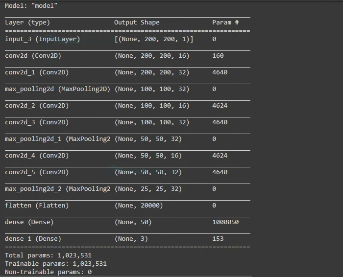
Firstly we will have an Input layer with the shape of our image array i.e.( Image Height , Image Width , Image Depth ) where our depth will be 1 as we have Grayscale image data. This input is then passed into the Convolution-pooling layer with ‘relu’ activation function. As we have discussed earlier about convolution layers.

Pooling layer is useful to get the maximum value from the feature that we have got using a filter. Later we will use a flatten layer to reshape our tensors of our network in order to have the shape that is equal to the number of elements i.e. number of labels in our case.

Code:

#Input with the shape of (200,200,1)
inputt = Input(shape=(im_size,im_size,1))

#convolutional layer with maxpooling
x=Conv2D(16, (3, 3),activation='relu',strides=(1, 1),padding='same')(inputt)
x=Conv2D(32, (3, 3),activation='relu',strides=(1, 1),padding='same')(x)
x=MaxPool2D((2, 2))(x)
x=Conv2D(16, (3, 3),activation='relu',strides=(1, 1),padding='same')(x)
x=Conv2D(32, (3, 3),activation='relu',strides=(1, 1),padding='same')(x)
x=MaxPool2D((2, 2))(x)

x=Conv2D(16, (3, 3),activation='relu',strides=(1, 1),padding='same')(x)
x=Conv2D(32, (3, 3),activation='relu',strides=(1, 1),padding='same')(x)
x=MaxPool2D((2, 2))(x)

#Flatten layer
x=Flatten()(x)
x=Dense(50, activation='relu')(x)

And finally create a Dense(fully connected) layer for output with the shape equal to the number of labels i.e. in our case 3 (normal,bacteria,virus) and ‘softmax’ activation function. Then Initialize Model Class with network input and Dense layer as output.

We can also see a summary of our build model.

Code:

#Dense (output) layer with the shape of 3(total number of labels)
outputt=Dense(3, activation='softmax')(x)

#create model class with inputs and outputs
model= Model(inputs=inputt,outputs=outputt)
#model summary
model.summary()

Output:

7) Train the Model

After constructing the model now it’s time to train our model. We will be using categorical cross-entropy loss function and Adam optimizer with the learning rate of 1e-3 (0.001) on a batch size of 32 for 50 epochs.

Code:

#epochs for model training and learning rate for optimizer
epochs = 50
learning_rate = 1e-3

#using Adam optimizer to compile or build the model
optimizer = Adam(learning_rate=learning_rate)
model.compile(optimizer=optimizer,
      loss='categorical_crossentropy',
      metrics=["accuracy"])
#fit the training generator data and train the model
hist = model.fit(train_generator,
           steps_per_epoch= x_train.shape[0] // batch_size,
           epochs= epochs,
           validation_data= test_generator,
           validation_steps= x_test.shape[0] // batch_size)

#Accuracy Graph
plt.figure(figsize=(8,6))
plt.title('Accuracy scores')
plt.plot(hist.history['accuracy'])
plt.plot(hist.history['val_accuracy'])
plt.legend(['acc', 'val_acc'])
plt.show()

#Loss Graph
plt.figure(figsize=(8,6))
plt.title('Loss value')
plt.plot(hist.history['loss'])
plt.plot(hist.history['val_loss'])
plt.legend(['loss', 'val_loss'])
plt.show()

Output:

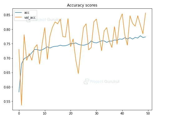
From the above graph you can see that the model’s performance is good, though at some point accuracy and loss value fluctuates. Also we can see there is no overfitting, as we have used Data Augmentation Technique.

Save the model in order for the prediction process

Code:

#Save the model for prediction
model.save("s2s")

Output:

8) Evaluating the model’s performance

Now, let’s see how our model performed by testing its accuracy with test data. For this we’ll be using a confusion matrix. Our matrix structure will contain Actual data i.e. ‘y_test’ (actual value of ‘x_test’) and Predicted data i.e. ‘y_pred’ (predicted value of ‘x_test’). Also we need to transform our predicted value back to original labels i.e. ‘bacteria’,’normal’,’virus’. Finally plot the matrix using ‘seaborn’ which is a statistical data visualization library of python.

Code:

#ProjectGurukul Pneumonia Detection
model = load_model("s2s")
labels = ['bacteria','normal','virus']

#confusion matrix
y_pred = model.predict(x_test)
#transforming label back to original
y_pred = encoder.inverse_transform(y_pred)

#matrix of Actual vs Prediction data
c_matrix = confusion_matrix(y_test, y_pred)
plt.figure(figsize=(8,8))
plt.title('Confusion matrix',fontsize=14)
sns.heatmap(
  c_matrix, xticklabels=labels,yticklabels=labels,
  fmt='d', annot=True,annot_kws={"size": 14}, cmap='Reds')
plt.xlabel("Predicted",fontsize=12)
plt.ylabel("Actual",fontsize=12)
plt.show()

Output:

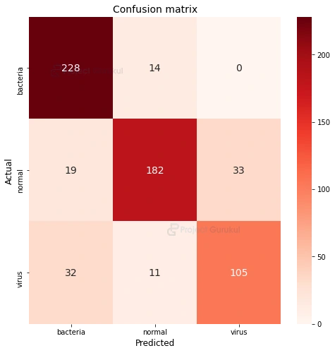
As you can see from the above matrix, out of 242 samples of bacteria images, 228 images were predicted as bacteria, out of 148 samples of virus images, 105 images were predicted as virus. But also you can see 32 virus images were predicted as bacteria as both the types of pneumonia are hard to differentiate. Thus, we can say our model has performed well and you can also increase its accuracy by changing some parameters.

9) Prediction

Finally display the ‘x_test’ images along with the Actual label and Predicted label.

Code:

for i in range(230,280,3):
pred = model.predict(x_test)[i]

#Display the x-ray image
cv2.imshow("ProjectGurukul",x_test[i])

#uncomment below line only when working on google colab
#cv2_imshow(x_test[i])

print("Actual :",y_test[i]," Predicted :",labels[np.argmax(pred)])

Pneumonia Detection Deep Learning Output:

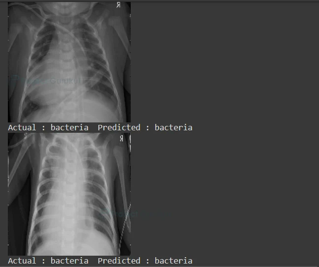
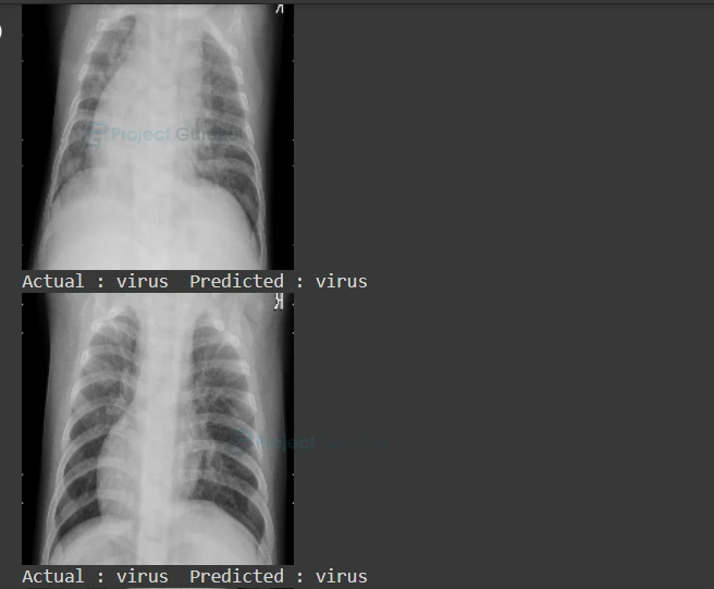
As you can see, we got our predicted label right. Our model accuracy is 80%. You can improve accuracy by adding convolutional layers or by changing the batch size.

Summary

In this Deep Learning Pneumonia Detection project, we have developed a model which predicts if a given x-ray of a person has pneumonia or not, if yes then whether it is caused by bacteria or virus using the Convolutional Neural Network.