Machine Learning Lung Cancer Detection using CNN

Lung cancer affects millions worldwide, posing a significant health challenge. It is characterized by abnormal cell growth within the lungs, often leading to life-threatening consequences. Detecting lung cancer at the early stages can help in saving lives.

There are three main types of lung cancer namely

1. Adenocarcinoma: This type of cancer starts in the cells that line the inner parts of certain organs, like the lungs. Adenocarcinoma tends to form in glands that produce mucus, which can happen in different parts of the body. In the lungs, it often starts in the outer regions.

2. Large cell carcinoma: This is a type of lung cancer that tends to grow and spread quickly. It gets its name from the appearance of the cancer cells under a microscope—they’re larger and look different from other types of lung cancer cells.

3. Squamous cell carcinoma: Squamous cell carcinoma starts in the flat cells that line the airways of the lungs. These cells are called squamous cells. This type of cancer usually forms in the central part of the lungs, around the bronchi. It’s often linked to smoking and can sometimes cause a cough, chest pain, or breathing difficulties.

In this article, we will learn how to develop a lung cancer detection system using convolutional neural networks.

Prerequisites For Machine Learning Lung Cancer Detection Project

• A good understanding of Python
• Jupyter Notebook
• Creating and managing Python environments

Download Machine Learning Lung Cancer Detection Project

Please download the source code of the Machine Learning Lung Cancer Detection Project from the following link: Machine Learning Lung Cancer Detection Project Code.

What are we going to build?

By the end of this Machine Learning Lung Cancer Detection Project, we aim to build a convolutional neural network that can classify CT scans of lungs into 4 different diagnoses:

• Adenocarcinoma
• Large cell carcinoma
• Squamous cell carcinoma
• Normal

Please download the dataset by using this link: Dataset

Steps to Develop the Machine Learning Lung Cancer Detection System

Step 1: Importing the necessary libraries

First, we will create a new Python file called ‘model.py’ or a Python notebook file called ‘model.ipynb’ and import the following libraries.

Code:

import matplotlib.pyplot as plt
import tensorflow as tf
from tensorflow.keras.models import Sequential
from tensorflow.keras.preprocessing.image import ImageDataGenerator
from tensorflow.keras.layers import Dense, Flatten,Dropout,BatchNormalization
from tensorflow.keras.models import Model
from tensorflow.keras.optimizers import Adam
from tensorflow.keras.applications.resnet50 import ResNet50, preprocess_input
from tensorflow.keras.callbacks import EarlyStopping, ModelCheckpoint
from tensorflow.keras.utils import plot_model

Explanation:

• os: Used to manage file directories
• matplotlib.pyplot: Used to plot graphs and images
• tensorflow: Used to build the deep learning model
• Sequential: Allows developers to specify that an input must pass through a series of neural layers until it reaches the output
• ImageDataGenerator: Helps create batches of image data with data augmentation
• ResNet50: A variation of the ReseNet architecture, a popular CNN model that we will use to initialize our neural network
• preprocess_input: Modifies the input to the format required by the model
• Model: Groups all the defined neural layers into a single object
• Adam: A popular optimization algorithm that improves accuracy and reduces loss
• EarlyStopping: Helps prevent overfitting, the machine learning concept where the model performs well only with the training data but does perform well with unseen data. EarlyStopping works by monitoring a metric across the entire training period. It interrupts the training when no significant change has occurred over several epochs.
• ModelCheckpoint: Used to save a model at an interval, from which we can load the model and continue training later.
• plot_model: Helps to generate a plot of the model architecture

Step 2: Specifying paths to the dataset

Next, we must specify the paths to the dataset we downloaded into the program to load the dataset.

Ensuring the dataset is extracted into the same root folder as the Python file is essential.

Code:

model_name = "Lung Cancer Detection using Convolutional Neural Network"
home = os.getcwd()
path = f'{home}\\archive\\Data\\'
train_path = path + 'train\\'
val_path = path + 'valid\\'
test_path = path + 'test\\'
splits = ['Train', 'Valid', 'Test']
input_shape = (224, 224, 3)
classes = 4
target_size = (224, 224)
batch_size = 32

Explanation:

• model_name: Specify the current project’s name, which will be useful for generating and saving files.
• home: Using os.getcwd(), get the path of the current working directory
• path: Define the path of the dataset
• train_path: Define the training path of the dataset
• val_path: Define the validation path of the dataset
• splits: Creating a list of this project’s dataset splits – training and validation. This information will be helpful later on.
• input_shape: Defining the input shape of the training images
• classes: Defining the total number of classes in this dataset – 5
• target_size: Defining the final target_size of the images that TensorFlow’s ImageDataGenerator will generate
• batch_size: When training a model with substantial data, batches are employed. The batch size refers to the number of training instances for a particular batch.

Step 3: Initializing the image data generators

We must define the training, testing and validation image data generators to load the images. These generators help to load images into the batches specified earlier upon completing the data augmentation.

Code:

train_datagen = ImageDataGenerator(
    dtype='float32',
    preprocessing_function=preprocess_input,
    rotation_range=20,
    width_shift_range=0.2,
    height_shift_range=0.2,
    shear_range=0.2,
    zoom_range=0.2,
    horizontal_flip=True,
    vertical_flip=False
)

val_datagen = ImageDataGenerator(
    dtype='float32',
    preprocessing_function=preprocess_input
)

test_datagen = ImageDataGenerator(
    dtype='float32',
    preprocessing_function=preprocess_input
)

train_generator = train_datagen.flow_from_directory(
    train_path,
    target_size=target_size,
    batch_size=batch_size,
    class_mode='categorical',  
)

test_generator = test_datagen.flow_from_directory(
    test_path,
    target_size=target_size,
    batch_size=batch_size,
    class_mode='categorical',
)

validation_generator = val_datagen.flow_from_directory(
    val_path,
    target_size=target_size,
    batch_size=batch_size,
    class_mode='categorical',
)

Explanation:

• train_datagen: Initialize the training image data generator and apply augmentation functions to the images
• train_generator: Specify the path and final outputs of the training image data generator
• Similarly, repeat the process for the validation and testing of images.

Step 4: Initializing the Model

Now, we will build the neural network using TensorFlow’s pre-defined ResNet50 model as the base model and add more layers.

Code:

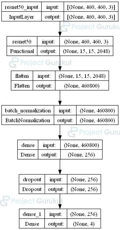
base_model = ResNet50(include_top=False, pooling='av', weights='imagenet', input_shape=(input_shape))
for layer in base_model.layers:
    layer.trainable = False
model = Sequential()
model.add(base_model)
model.add(Flatten())
model.add(BatchNormalization())
model.add(Dense(256, activation='relu'))
model.add(Dropout(0.5))
model.add(Dense(classes, activation='softmax'))
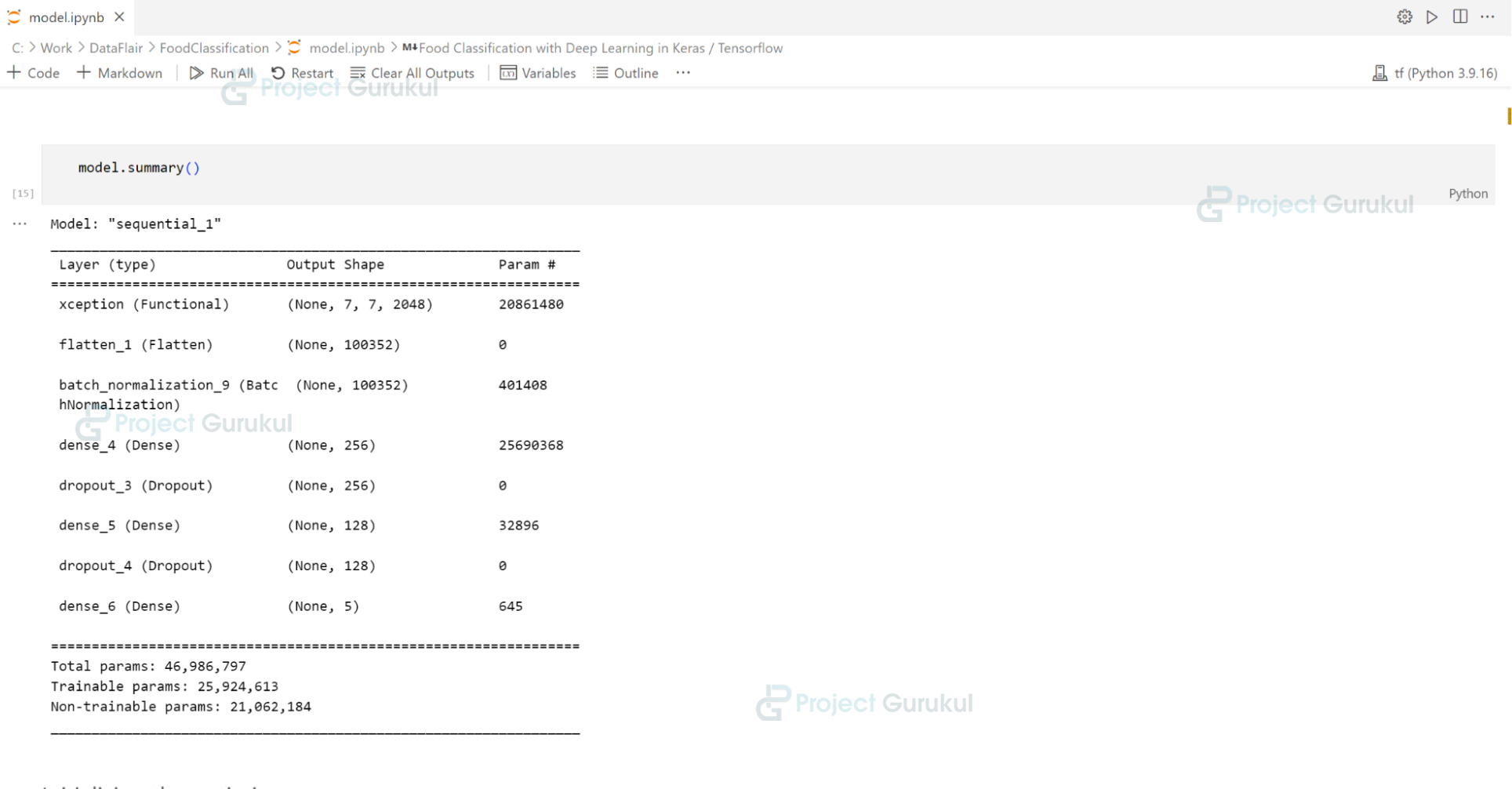
model.summary()
plot_model(model,to_file=f"{model_name}", show_shapes=True, show_layer_names=True)

Summary of the Lung Cancer Detection Model

Architecture Diagram of the Lung Cancer Detection Model

Explanation:

• base_model: Define ResNet50 to be the base model of our neural network, using the famous ‘imagenet’ weights
• layer.trainable: To retain the knowledge from previous weights during the training stage, we set their trainable attribute to false.
• Sequential: Using the base_model, we define our model by adding a few more layers. First, we add the Flatten() layer to reduce the dimensionality of the previous CNN layers from a 3D tensor to a 1D tensor to make it easier for training. Next, we add a BatchNormalization() layer to normalize the data, allowing for stable training. Dense layers are fully connected layers that add a layer with a specified number of neurons. For this model, a single dense layer of 256 neurons is enough to train it with good accuracy. While training, we integrate dropout layers to randomly deactivate a specified percentage of units, thereby reducing the risk of overfitting.
• model.summary: Displays the model architecture
• plot_model: Downloads the image of the model architecture
• optimizer: Initializes the Adam optimizer, which the model will use while training

Step 5: Compiling the Model

The next step is to compile the model before we start the training stage.

Code:

model.compile(loss='categorical_crossentropy',optimizer=optimizer,metrics=['accuracy'])
optimizer = tf.keras.optimizers.Adam()
checkpoint = ModelCheckpoint(
    filepath=f'{model_name}.h5',
    monitor='val_loss',
    save_best_only=True,
    verbose=1
)
earlystop = EarlyStopping(
    patience=10,
    verbose=1
)

Explanation:

• model.compile: Here, we specify the loss function, optimizer, and metrics to track. We use loss functions to measure the disparity between the model’s predicted and actual values. We use categorical crossentropy as it is one of the most popular loss functions for multi-class classification. To track the progress of our model’s training, we will be using ‘accuracy.’
• checkpoint: Saves the model into a specified file whenever the validation loss improves over the training time.
• earlystop: To avoid overfitting the model, we use EarlyStopping with patience of 10 epochs. Epochs refer to one complete pass by the model through the entire training dataset.

Step 6: Training the Model

With the compilation of the model complete, we can now initiate the training process.

Code:

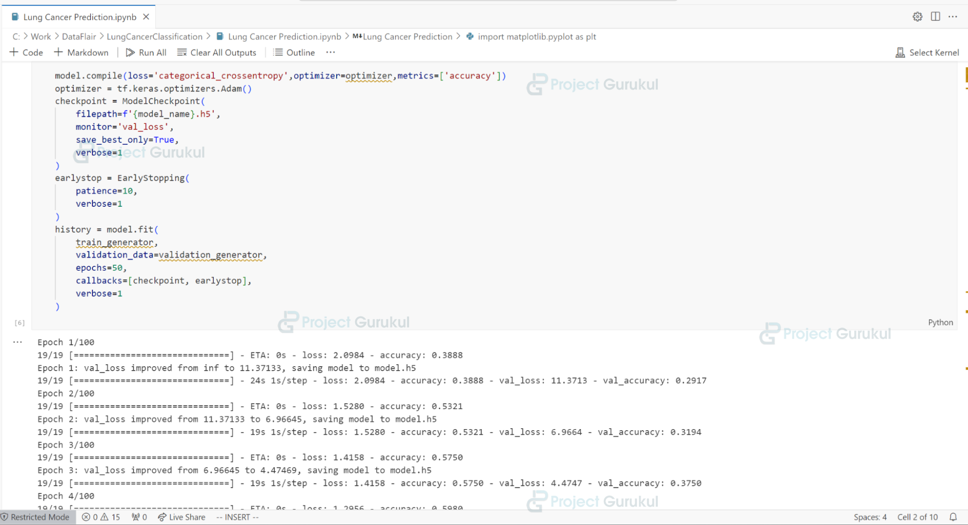
history = model.fit(
   train_generator,
   validation_data=val_generator,
   epochs=50,
   callbacks=[checkpoint, earlystop],
   verbose=1
)
history = model.fit(
    train_generator,
    validation_data=validation_generator,
    epochs=100,
    callbacks=[checkpoint, earlystop],
    verbose=1
)

Training the Lung Cancer Detection Model

Explanation:

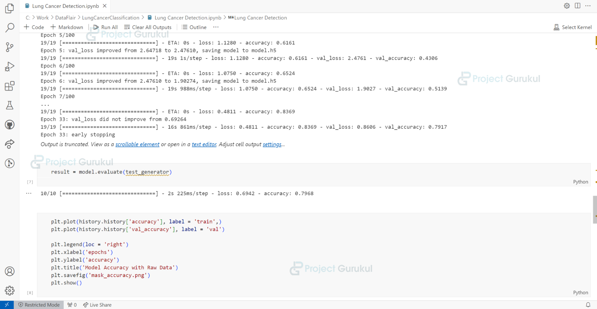
• history: We fit the model with the training images generated while simultaneously validating the data with the validation images generated. We train the model for 50 epochs; however, it will finish sooner than that, thanks to early stopping.

Step 7: Testing the Model

Now that the model has successfully finished training, we can test the accuracy with the dataset’s testing data.

Code:

result = model.evaluate(test_generator)

Evaluating the Lung Cancer Detection Model

Explanation:

• model.evaluate: We perform the testing function on the trained model using the test data.

Step 8: Plotting the accuracy and loss

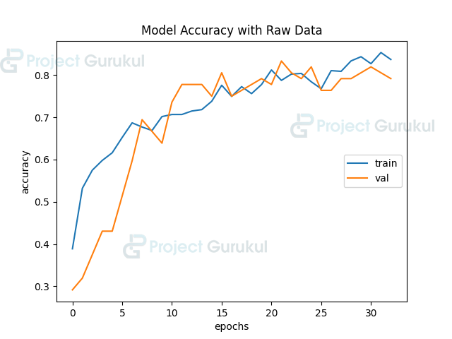
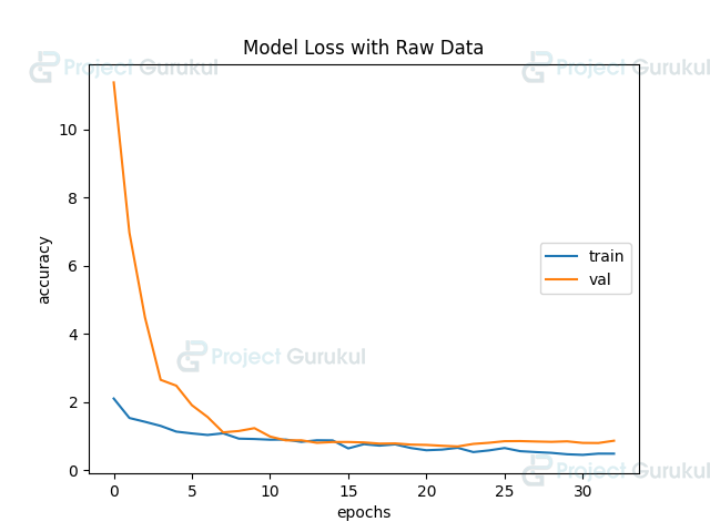
The model has finished training and has successfully saved into a .h5 file. We can then load it into another application, as per our requirements. Let’s plot the accuracy and loss to visualize our model’s performance. We aim to generate two images, one containing the accuracy and validation accuracy, the other containing loss and validation loss.

Code:

plt.plot(history.history['accuracy'], label = 'train',)
plt.plot(history.history['val_accuracy'], label = 'val')

plt.legend(loc = 'right')
plt.xlabel('epochs')
plt.ylabel('accuracy')
plt.title('Model Accuracy with Raw Data')
plt.savefig(f'images\\accuracy.png')
plt.show()

plt.plot(history.history['loss'], label = 'train',)
plt.plot(history.history['val_loss'], label = 'val')

plt.legend(loc = 'right')
plt.xlabel('epochs')
plt.ylabel('accuracy')
plt.title('Model Loss with Raw Data')
plt.savefig(f'images\\loss.png')
plt.show()

Explanation:

• metrics: We declare a list with the metrics that need to be visualized, such as accuracy and loss. To reduce the overall length of our code, we will use a ‘for’ loop and the Python concept of ‘f-strings’.
• We will generate the graphs using matplotlib. Using a ‘for’ loop, first we will apply plt.clf() to clear the current figure. Using ‘history’, we plot the current metric and give them appropriate labels. The labels appear on the right side of the image under the ‘legend’ column. The x-axis denotes the number of epochs, while the y-axis represents the percentage of the plotted metric. Thus, we assign appropriate labels to them. Finally, we give the plots relevant names and save them as a ‘.png’ file under the ‘images’ folder.

NOTE: To meet permission requirements, it is advisable to manually create an ‘images’ folder under the same root directory as the ‘.py’ file.

Accuracy of the Lung Cancer Detection Model

Loss of the Lung Cancer Detection Model

Conclusion

This project taught us how to build a Lung Cancer Detection model using Python and TensorFlow. Using the pre-trained ResNet50 model, we added a dense layer with 256 neurons and a dropout layer. We trained the model for 50 epochs, implementing early stopping to prevent overfitting. We saved the model to a ‘.h5′ file, making it easily usable in other applications.

Finally, we visualized our model’s performance by plotting the accuracy and loss graphs over the training period. The model’s ability to analyze medical imaging data swiftly and accurately aids doctors in making informed decisions about whether patients are suffering from lung cancer and which type of lung cancer it may be.

In conclusion, this Python and TensorFlow-based lung cancer detection system can reduce doctors’ and oncologists’ workloads by making it simpler to determine whether a patient has cancer.