Market Basket Analysis using Apriori Algorithm

With this Machine Learning Project, we will be doing market-basket analysis. For this project, we are using the Apriori algorithm.

So, let’s build this system.

Market-Basket Analysis System

One of the most important methods used by major retailers to identify correlations between products is market basket analysis. It operates by looking for product combinations that regularly appear together in transactions. Put another way, it enables businesses to discover connections between the products that customers purchase. In order to uncover strong rules that are found in transaction data, the association rules are frequently employed to analyze retail basket or transaction data.

People today purchase everyday necessities from the nearest supermarket. Numerous supermarkets provide different products to their customers. The positioning of the merchandise is a challenge that many shops have. They do not know the customer’s purchasing preferences; thus, they are unsure of what products to group together in their store. Shop owners can put products that frequently occur together close to one another by using this application to identify the strong correlations between the items. Additionally, choices are made on which item to stock more of, cross-selling, up-selling, and shelf placement in stores.

A modelling method known as “affinity analysis” or “market basket analysis” can help determine which products are most likely to be bought together. The market basket issue takes a lot of things into account. The marketer learns the items the consumer has purchased collectively after the buyer purchases the subset of goods that best suits his demands. Therefore, the marketer places things in various spots using this knowledge. As an illustration, when someone purchases a packet of milk, they frequently also purchase bread. It implies milk = bread. Locating things inside a store is decided using a market basket analysis. A consumer is more likely to purchase butter if he also purchases a packet of bread. Customers would be persuaded to purchase one item with the other if bread and butter were kept close together at a store.

There are numerous market prospects offered by data mining. For a firm to survive in this cutthroat market, decision-making and comprehending customer behavior have become crucial and difficult problems. In order to obtain a competitive advantage, the firm faces hurdles in extracting data from its extensive client datasets. According to Yanthy et al. in their paper, data mining aims to uncover hidden knowledge from data. Various algorithms have been proposed to accomplish this. Still, the problem is that not all generated rules are typically interesting—only a small portion of them would interest any given user.

Rakesh Agarwal used the Apriori algorithm in his research which shows very great results. Apriori was the first associative algorithm to be developed, and it has since been utilized as a technique in creating the association, classification, and associative classification algorithms. The Apriori method counts transactions in a level-wise, breadth-first manner. Prior knowledge of frequent item set properties is used in the apriori algorithm. In Apriori, n-item sets are used to explore (n+1)-item sets using an iterative process known as a level-wise search. Here, the Apriori property is employed to increase the effectiveness of the level-wise production of frequent item sets. A frequent item set’s non-empty subsets must all be frequent according to the a priori property.

Apriori Algorithm

The goal of association rule discovery is to create if-then rules based on the itemsets x defined in the preceding subsection. “If a market basket has orange juice, then it also contains bread,” is an illustration of such a rule. This section discusses the Apriori algorithm for locating all frequent item sets. One of the most significant data mining techniques is the traditional Apriori method. It uses a breadth-first search methodology to find all frequent 1-itemsets first, followed by 2-itemsets, and then larger and larger frequent itemsets. It first examines how to determine the support for any itemset and store the data in memory, then discusses the actual apriori algorithm, and finally identifies the size of candidate item sets, which allows for an estimation of computational time because the size of the candidates influences the complexity of the algorithm.
Using an analysis of data collection, the Apriori algorithm determines which item combinations are most common. It is the foundation for many algorithms used to solve data mining issues. The most well-known challenge is finding the association rules that apply in a basket-item relation. A large item set can only be considered large if all its subgroups have large item sets. You can think about the sets of items that have the least amount of support. A frequent item set can be used to build association rules.

Knowledge discovery in databases, or KDD, is the process of finding knowledge in data and the application of data mining techniques. One of the KDD process’s steps is data mining. It employs a suitable algorithm in accordance with the KDD process’s objective of finding patterns in data. Finding patterns and links via data mining is kind of a crucial process. It is a process that uses artificial intelligence methods, neural networks, and sophisticated statistical tools like cluster analysis to identify trends, patterns, and linkages that could otherwise go undetected in vast datasets kept in data warehouses. There are many applications for data mining, both in the public and private sectors. Knowledge discovery in databases, or KDD, is the process of finding knowledge in data and the application of data mining techniques.

Project Prerequisites

The requirement for this project is Python 3.6 installed on your computer. I have used a Jupyter notebook for this project. You can use whatever you want.
The required modules for this project are –

1. Numpy(1.22.4) – pip install numpy
2. Tensorflow(2.9.0) – pip install TensorFlow
3. OpenCV(4.6.0) – pip install cv2

That’s all we need for our project.

Market Basket Analysis Project

We have provided the dataset and market basket analysis project code that will be required in this project. We will require a csv file & code for this project. Please download the dataset and source code from the following link: Market Basket Analysis Project

Steps to Implement

1. Import the modules and the libraries. For this project, we are importing the libraries numpy, pandas, and sklearn. Here we also read our dataset and we are saving it into a variable.

import numpy as np #importing the numpy library we will need in this project
import pandas as pd #importing the pandas library we will need in this project
from mlxtend.frequent_patterns #import apriori #importing our apriori algorithm from mlxtend
from mlxtend.frequent_patterns import association_rules #import association from mlxtend.frequent
 
import time #importing the time function from python library
 
df = pd.read_csv(‘dataset.csv') #importing our dataset Online RetailShop Germany which is a csv file
df.head() #printing the head of our dataset file

2. Installing the mlxtend library

!pip install mlxtend

3. Here we are reading our dataset. We are also removing the spaces and checking if any value is missing.

missing_value = ["NaN", "NONE", "None", "nan", "none", "n/a", "na", " "] #making an array for possible keyword of missing values
df = pd.read_csv('OnlineRetailShopGermany.csv', na_values = missing_value) #read our dataset file and passing our missing value array
print (df.isnull().sum()) #here we are checking if there is any null value in the dataset.

4. Here we are using the strip function to strip the text in the description column.

df['Description'] = df['Description'].str.strip() #here we are using the strip fnction of string in python to strip the Description column
df.Description.value_counts(normalize=True)[:10] #here we are printing the count of the description value.

5. Here we are doing pre-processing our dataset. After that, we are selecting duplicate rows excerpt first occurrence based on all columns.

 
df.drop(df[df['Description'] == 'POSTAGE'].index, inplace = True) #here we are dropping the Description column and we are passing the inplace = True
 
# Select duplicate rows except first occurrence based on all columns
duplicateRows = df[df.duplicated()] #selecting the duplicate columns
# print(duplicateRows.head())
df = df.drop_duplicates() #dropping the duplicates columns in our dataset

6. Here we are sorting the dataset according to Quantity using the groupby function.

 
df2 = (df.groupby(['InvoiceNo', 'Description'])['Quantity']
          .sum().unstack().reset_index().fillna(0)
          .set_index('InvoiceNo')) #sorting the dataset according to Quantity and in this we are using the groupby function.
 

7. Here, we are defining the function convertToZeroOne. In this, we are passing the x values, and we are checking if x<=0 then we are converting it to 0, i.e. converting the negative values to 0 and the non-negative values to 1. Finally, we plot the curve.

def convertToZeroOne(x): #defining our converting function
    if x <= 0: #checking if x is less than or equal to zero
        return 0 #returning 
    if x >= 1: #if x=1 
        return 1 # we are returning 1
 
df3 = df2.applymap(convertToZeroOne) #we are using the function convertToZeroOne
 
start_time = time.time() #calculating the start time
frequent_itemsets = apriori(df3, min_support=0.04, use_colnames=True)#using the apriori algorithm and passing the dataset 
end_time = time.time() #calculating the end time
Frequent_itemsets #printing the dataset.
 
rules = association_rules(frequent_itemsets, metric="lift", min_threshold=1) #using the association rules function and passing the dataset to it.
rules.head()#printing the rules dataset.
rules[(rules['lift'] >= 0.5) & (rules['confidence'] >= 0.3)] #checking if confidence >=0.3 and lift >=0.5

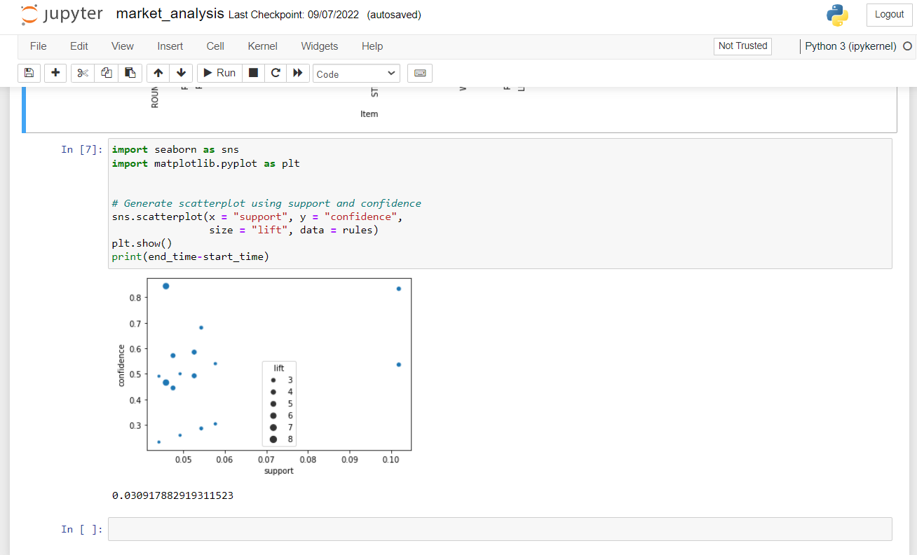
8. Importing the seaborn library and matplot library to plot a scatter plot graph.

import seaborn as sns#importing the seaborn library
import matplotlib.pyplot as plt#importing the matplotlib 
 
sns.scatterplot(x = "support", y = "confidence", 
                size = "lift", data = rules)#using sns to plot a scatter plot curve
plt.show() #plotting the graph

Summary

In this Machine Learning project, we are doing a market-basket analysis. For this project, we are using the Apriori Algorithm. We hope you have learned something new from this project.