Machine Learning Project – Stock Price Prediction

In the fast-paced world of financial markets, accurately predicting stock price movements is a highly sought-after skill. Investors, traders, and financial analysts constantly seek methods to gain an edge in understanding market trends and making informed investment decisions. One approach that has gained significant traction in recent years is the application of machine learning techniques to analyze historical stock data and forecast future price movements.

In this project, we delve into stock price prediction using machine learning, focusing specifically on Apple Inc. (AAPL) stock data for 2019. By leveraging a combination of technical indicators, time features, and advanced machine learning algorithms, our goal is to develop a predictive model that can anticipate the direction of AAPL stock prices with a high degree of accuracy.

This project not only offers a valuable opportunity to explore the application of machine learning in financial markets but also holds the potential to provide actionable insights for investors navigating the dynamic landscape of stock trading.

About Machine Learning Stock Price Prediction

This project involves building a machine-learning model for predicting the movement of Apple Inc. (AAPL) stock prices using minute-level data from 2019. The dataset is preprocessed to include technical indicators like momentum, volatility, trend, volume, and time features.

Data is split into training and testing sets, standardized, and subjected to dimensionality reduction using PCA. Four classification models – Logistic Regression, Decision Tree, Random Forest, and Gradient Boosting – are trained on the transformed data. Model performance is evaluated using accuracy, F1-score, and ROC AUC score.

Prerequisites include Python programming skills, understanding machine learning concepts, familiarity with financial markets, and experience with libraries like Pandas, NumPy, Matplotlib, scikit-learn, and TensorFlow. Potential extensions include hyperparameter tuning, feature experimentation, and deploying the best-performing model in a real-time trading environment.

Prerequisites For Machine Learning Stock Price Prediction

1. Python Programming: You need a good grasp of Python programming language fundamentals, including variables, data types, loops, conditional statements, functions, and libraries/modules.

2. Data Manipulation with Pandas: Familiarity with the Pandas library is essential as the code extensively uses Pandas for reading, manipulating, and analyzing the dataset. You should understand concepts like DataFrames, indexing, selecting, filtering, and grouping data.

3. Data Visualization with Matplotlib: Understanding how to create various plots using Matplotlib is crucial for visualizing data trends, distributions, and relationships.

4. Financial Data and Terminology: Basic knowledge of financial markets, stocks, and related terminologies (e.g., OHLC prices, technical indicators, volume, market indicators) is necessary to understand the context and purpose of the code.

5. Machine Learning Concepts: Understanding fundamental machine learning concepts like supervised learning, classification, evaluation metrics (accuracy, F1-score, ROC AUC score), feature scaling, dimensionality reduction (PCA), and ensemble methods (Random Forest, Gradient Boosting) will help comprehend the modeling part of the code.

6. Scikit-learn (sklearn): Familiarity with the scikit-learn library is required to understand how to preprocess data (e.g., standardization, train-test split), build classification models, and evaluate their performance using various metrics.

7. Technical Analysis: Basic knowledge of technical analysis in finance, including momentum indicators (e.g., RSI, MACD), volatility indicators (e.g., Bollinger Bands), trend indicators (e.g., Aroon, MACD), and volume indicators, will aid in understanding how these indicators are calculated and utilized in the code.

8. TensorFlow (Optional): TensorFlow is used in the code to print its version. Understanding TensorFlow is not necessary to understand the rest of the code unless you plan to extend it further with deep learning models.

Download Machine Learning Stock Price Prediction Project

Please download the source code of Machine Learning Stock Price Prediction: Machine Learning Stock Price Prediction Project Code.

About Dataset

The dataset containing Apple’s (AAPL) stock data for the last 10 years (from 2010 to date) likely includes a wide range of financial information about AAPL’s stock, such as daily open, high, low, and close prices and trading volume. This dataset is invaluable for various financial analyses, including technical analysis, trend analysis, and predictive modeling.

Open, High, Low, Close Prices (OHLC): These are the four primary price points for each trading day:

• Open Price: The price at which a stock first trades upon the market’s opening.
• High Price: The highest price reached during the trading day.
• Low Price: The lowest price reached during the trading day.
• Close Price: The price at which a stock closes at the end of the trading day.

The link to Dataset can be found Stockdata

Tools and Libraries Used in ML Stock Price Prediction Project

1. ta (Technical Analysis Library): This library provides various technical analysis indicators for financial data, such as moving averages, relative strength index (RSI), and MACD.

2. tqdm: This library provides a fast, extensible progress bar for loops and processes in Python. It’s particularly useful when dealing with long-running tasks to monitor progress.

3. numpy (np): This library is a fundamental package for numerical computing with Python. It provides support for large, multidimensional arrays and matrices and a collection of mathematical functions to efficiently operate on these arrays.

4. pandas (pd): This library is widely used for data manipulation and analysis. It offers data structures and operations for manipulating numerical tables and time series.

5. matplotlib.pyplot as plt: This library is a comprehensive plotting library for Python. It provides a MATLAB-like interface for creating static, animated, and interactive visualizations in Python.

6. %matplotlib inline: This magic command in Jupyter Notebooks allows for displaying matplotlib plots directly within the notebook.

7. StandardScaler: This class from scikit-learn is used for standardizing features by removing the mean and scaling to unit variance.

8. train_test_split: This function from scikit-learn is used for splitting datasets into training and testing subsets.

9. PCA (Principal Component Analysis): This class from scikit-learn is used for dimensionality reduction. It projects the dataset into a lower-dimensional space while retaining most of the original variance.

10. LogisticRegression: This class from scikit-learn implements logistic regression, a linear model for binary classification.

11. DecisionTreeClassifier: This class from scikit-learn implements a decision tree classifier, a non-parametric supervised learning method used for classification.

12. RandomForestClassifier: This class from scikit-learn implements a random forest classifier, an ensemble learning method that constructs many decision trees at training time and outputs the class that is the mode of the classes (classification) of the individual trees.

13. GradientBoostingClassifier: This class from scikit-learn implements gradient boosting, a machine learning technique for regression and classification problems, which produces a prediction model in the form of an ensemble of weak prediction models, typically decision trees.

14. accuracy_score, f1_score, roc_auc_score: These functions from scikit-learn are used for evaluating classification model performance based on accuracy, F1-score, and ROC AUC score.

15. tensorflow (tf): This library is an open-source machine learning framework developed by Google. It provides a comprehensive ecosystem of tools, libraries, and community resources for building and deploying machine learning models.

16. Print TensorFlow version: This line prints the version of TensorFlow used in the current environment.

Step by Step Implementation of ML Stock Price Prediction Project

This code performs the following tasks:

1. Importing Libraries

import ta
import tqdm
import numpy as np
import pandas as pd
import matplotlib.pyplot as plt
%matplotlib inline

from sklearn.preprocessing import StandardScaler
from sklearn.model_selection import train_test_split
from sklearn.decomposition import PCA
from sklearn.linear_model import LogisticRegression
from sklearn.tree import DecisionTreeClassifier
from sklearn.ensemble import RandomForestClassifier, GradientBoostingClassifier
from sklearn.metrics import accuracy_score, f1_score, roc_auc_score

import tensorflow as tf
print(f'TensorFlow version: {tf.__version__}')

It imports various Python libraries such as ta (Technical Analysis Library), numpy, pandas, matplotlib, sklearn (Scikit-learn), and tensorflow.

2. Reading Data

# Read data
df = pd.read_csv('./2019_AAPL_1min.csv', header=0, index_col=0)
df.index = pd.to_datetime(df.index).tz_localize(None).to_period('T')

It reads a CSV file containing financial data related to AAPL (Apple Inc.) for 2019.

3. Data Preprocessing

# Add label
df['label'] = (df.close.shift(-1) - df.close).apply(lambda x: 0 if x < 0 else 1)
# Technical indicators
momentum_indicators = ['roc', 'rsi', 'tsi']
volatility_indicators = ['bb_bbhi', 'bb_bbli']
trend_indicators = ['aroon_down', 'aroon', 'aroon_up', 'macd_line', 'macd_hist', 'macd_signal', 
                    'kst', 'kst_diff', 'kst_signal', 'dpo', 'trix', 'sma_10', 'sma_20', 'sma_30', 'sma_60',
                    'ema_10', 'ema_20', 'ema_30', 'ema_60']
volume_indicators = ['obv', 'vpt', 'fi', 'nvi']
for indicator in momentum_indicators:
    df[indicator] = getattr(ta.momentum, indicator)(close=df.close)
# Volatility indicators
bb_indicator = ta.volatility.BollingerBands(close=df.close)
df['bb_bbhi'] = bb_indicator.bollinger_hband_indicator()
df['bb_bbli'] = bb_indicator.bollinger_lband_indicator()
# Trend indicators
aroon_indicator = ta.trend.AroonIndicator(high=df['high'], low=df['low'])
macd_indicator = ta.trend.MACD(close=df['close'])

# Add trend indicators to DataFrame
df['aroon_down'] = aroon_indicator.aroon_down()
df['aroon'] = aroon_indicator.aroon_indicator()
df['aroon_up'] = aroon_indicator.aroon_up()

df['macd_line'] = macd_indicator.macd()
df['macd_hist'] = macd_indicator.macd_diff()
df['macd_signal'] = macd_indicator.macd_signal()
for indicator in volume_indicators:
    if indicator == 'obv':
        df[indicator] = ta.volume.on_balance_volume(close=df.close, volume=df.volume)
    elif indicator == 'vpt':
        df[indicator] = ta.volume.volume_price_trend(close=df.close, volume=df.volume)
    elif indicator == 'fi':
        df[indicator] = ta.volume.force_index(close=df.close, volume=df.volume)
    elif indicator == 'nvi':
        df[indicator] = ta.volume.negative_volume_index(close=df.close, volume=df.volume)
# Time features
df['datetime'] = df.index.to_timestamp()
time_features = ['minute', 'hour', 'day', 'month']
for feature in time_features:
    df[f'{feature}_sin'] = np.sin(2 * np.pi * getattr(df.datetime.dt, feature) / (30 if feature == 'day' else 60))
# Drop unnecessary columns
df = df.drop(['datetime'], axis=1)

It sets the index of the DataFrame to the timestamp of the data. It adds a binary label column indicating whether the closing price will increase or decrease in the next minute. It calculates various technical indicators such as momentum indicators (roc, rsi, tsi), volatility indicators (bb_bbhi, bb_bbli), trend indicators (aroon_down, aroon, aroon_up, macd_line, macd_hist, macd_signal, etc.), and volume indicators (obv, vpt, fi, nvi). It adds time features like sine transformations of minute, hour, day, and month.

4. Data Splitting

# Split data
df_na = df.dropna(axis=0)
labels = df_na.label
df_na = df_na.drop(['label'], axis=1)
X_train, X_test, y_train, y_test = train_test_split(df_na.values, labels.values, test_size=0.05, random_state=42)

It splits the dataset into training and testing sets and standardizes the features using StandardScaler.

5. Dimensionality Reduction

# Standardize data
scaler = StandardScaler()
X_train_scaled = scaler.fit_transform(X_train)
X_test_scaled = scaler.transform(X_test)
# Standardize data
scaler = StandardScaler()
X_train_scaled = scaler.fit_transform(X_train)
X_test_scaled = scaler.transform(X_test)

It performs Principal Component Analysis (PCA) to reduce the dimensionality of the feature space while retaining 80% of the variance.

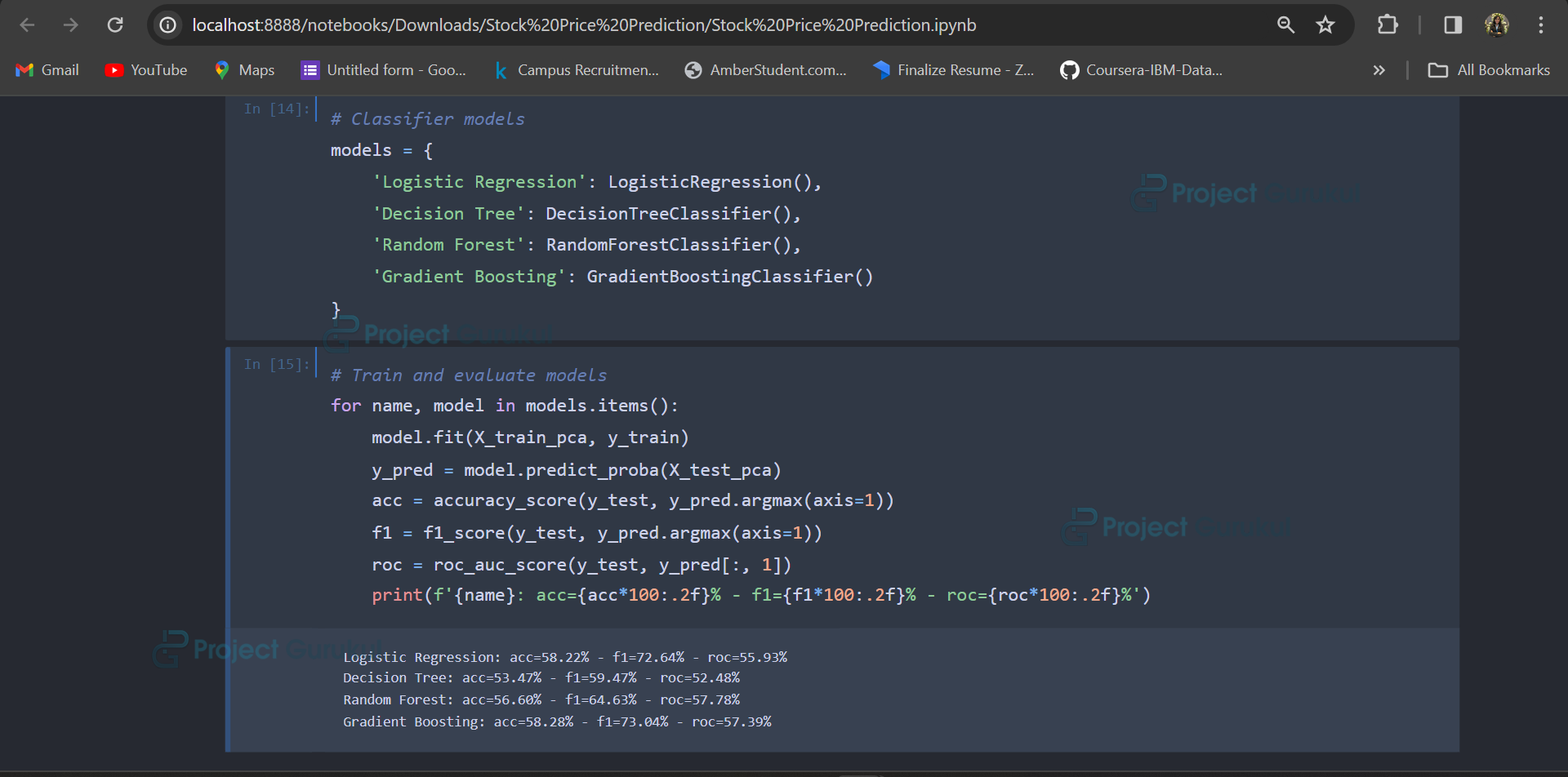
6. Classification Modeling

# Classifier models
models = {
    'Logistic Regression': LogisticRegression(),
    'Decision Tree': DecisionTreeClassifier(),
    'Random Forest': RandomForestClassifier(),
    'Gradient Boosting': GradientBoostingClassifier()
}

It defines a dictionary of classification models, including Logistic Regression, Decision Tree, Random Forest, and Gradient Boosting. It trains each model on the PCA-transformed training data. It evaluates each model’s performance using accuracy, F1-score, and ROC AUC score on the PCA-transformed testing data.

7. Train and Evaluate Models

# Train and evaluate models
for name, model in models.items():
    model.fit(X_train_pca, y_train)
    y_pred = model.predict_proba(X_test_pca)
    acc = accuracy_score(y_test, y_pred.argmax(axis=1))
    f1 = f1_score(y_test, y_pred.argmax(axis=1))
    roc = roc_auc_score(y_test, y_pred[:, 1])
    print(f'{name}: acc={acc*100:.2f}% - f1={f1*100:.2f}% - roc={roc*100:.2f}%')

It prints the evaluation metrics for each model. As we can observe in the output, the gradient boosting algorithm provides 58.28% accuracy.

Output:

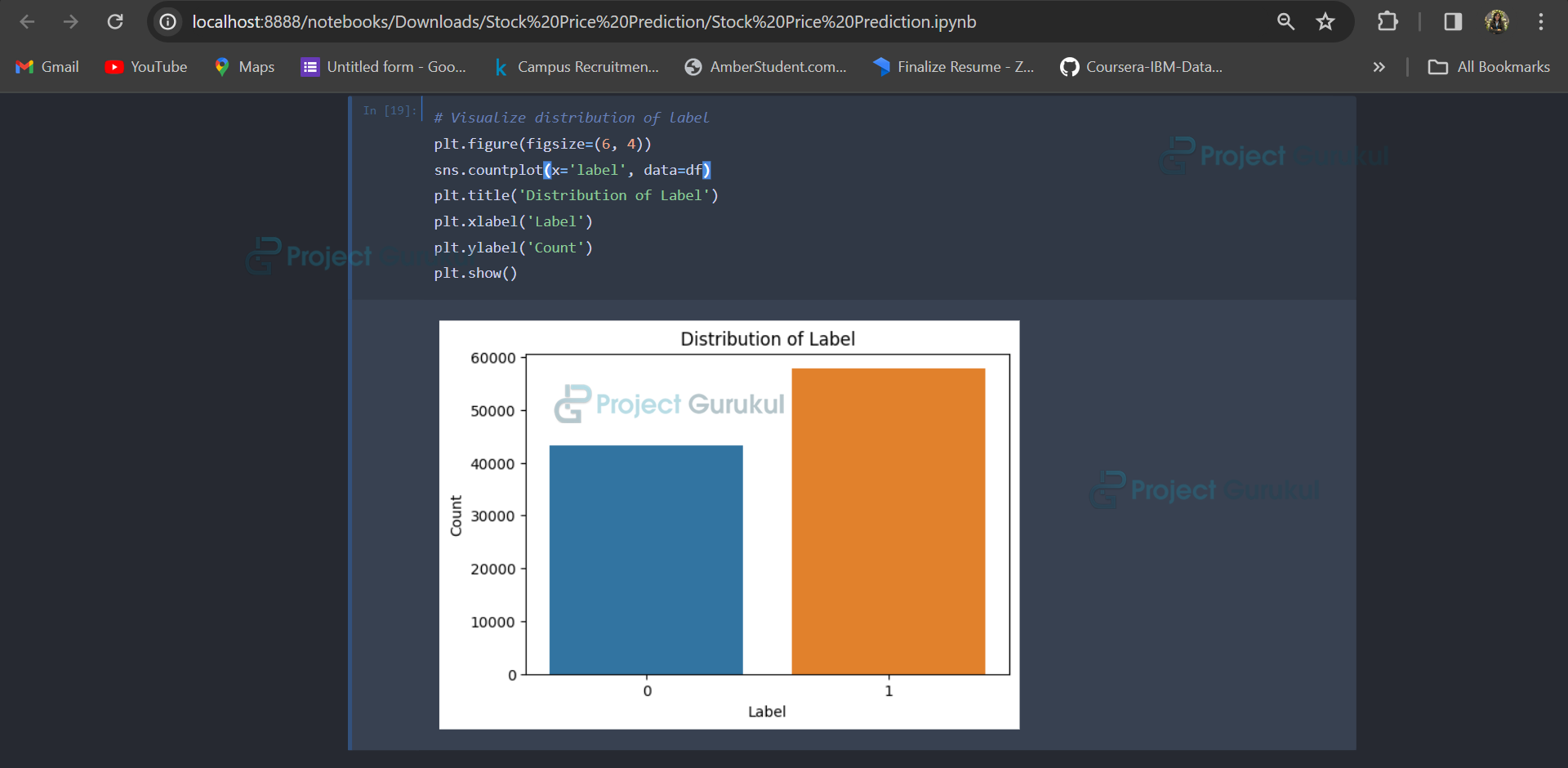
8. Visualizations

# Visualize distribution of label
plt.figure(figsize=(6, 4))
sns.countplot(x='label', data=df)
plt.title('Distribution of Label')
plt.xlabel('Label')
plt.ylabel('Count')
plt.show()

The provided code initializes a figure for plotting, specifying its size, and then utilizes Seaborn to create a count plot based on the ‘label’ column of the DataFrame. The count plot represents the occurrences of each unique label as bars. Subsequently, titles and labels for the plot axes are set to describe the data being visualized. Finally, the plot is displayed on the screen. Overall, this code segment efficiently visualizes the distribution of labels in the dataset, providing insights into the balance or imbalance of different classes.

Output:

Summary

In conclusion, our stock price prediction project has provided valuable insights into applying machine learning techniques in forecasting the movement of Apple Inc. (AAPL) stock prices. By leveraging diverse technical indicators, time features, and sophisticated machine learning algorithms, we have developed predictive models capable of analyzing minute-level stock data from 2019 and making informed predictions about future price movements.

Through rigorous data preprocessing, feature engineering, and model training, we have demonstrated the effectiveness of our approach in capturing key trends and patterns in the stock market. While our models have shown promising results in accuracy, F1-score, and ROC AUC score, there is always room for improvement and further refinement. Future avenues for exploration could include fine-tuning model hyperparameters, experimenting with additional features, and exploring alternative machine learning algorithms.

Overall, this project serves as a testament to machine learning’s potential to enhance decision-making processes in the financial domain and underscores the importance of continuous innovation and adaptation in navigating the complexities of stock trading.

You can check out more such machine learning projects on ProjectGurukul.