Machine Learning Project – Skin Cancer Classification

Skin cancer classification using Machine Learning involves the development of algorithms that can accurately identify and classify different types of skin lesions or moles based on medical images. The goal is to assist dermatologists and healthcare professionals in diagnosing skin cancer more quickly and accurately. This approach relies on leveraging large datasets of skin images, such as the HAM10000 dataset, to train machine-learning models.

The significance of skin cancer classification using Machine Learning lies in its potential to improve early detection and reduce the need for unnecessary biopsies. By providing automated and accurate diagnoses, these models can assist dermatologists in making more informed decisions about patient care. Additionally, this technology has the potential to expand access to skin cancer screening, particularly in regions with limited access to healthcare professionals, ultimately leading to better outcomes for patients.

Dataset

The dataset can be downloaded for free from Kaggle. This dataset is a comprehensive collection of dermatology images designed for skin cancer classification and research purposes. This dataset is particularly valuable for developing and training machine learning models to identify different types of skin lesions and assist in the diagnosis of skin cancer.

The dataset consists of high-quality clinical images of skin lesions, which have been carefully labeled and categorized into seven distinct classes representing various skin conditions. These classes include melanocytic nevi, melanoma, benign keratosis-like lesions, basal cell carcinoma, actinic keratoses, vascular lesions, and dermatofibroma.

Prerequisites For Machine Learning Skin Cancer Classification:

NumPy:

• Understanding of arrays and matrix operations.
• Ability to perform numerical computations efficiently.

Pandas

• Proficiency in handling and analyzing structured data.
• Understanding of DataFrames and Series.
• Ability to manipulate and preprocess seismic data, including cleaning, filtering, and transforming data.

Matplotlib:

• Knowledge of basic plotting techniques, including line plots, scatter plots, and histograms.
• Understanding of subplots for creating multiple plots in a single figure.
• Familiarity with advanced plot types, such as heatmaps, contour plots, and geographical visualizations.

Seaborn:

• Basic understanding of how to create various types of plots and charts in seaborn
• Familiarity with basics of Seaborn like syntax, functions, methods, etc

scikit-learn:

• Familiarity with machine learning concepts, such as supervised and unsupervised learning.
• Understanding of model selection, training, and evaluation procedures.

TensorFlow:

• Prior installation of TensorFlow, a popular deep learning framework, using tools like pip or conda.
• Familiarity with setting up the TensorFlow environment and importing TensorFlow libraries.

Deep Learning:

• A foundational understanding of deep learning principles is crucial.
• Familiarity with neural networks, convolutional neural networks (CNNs), and their architectures, such as convolutional layers, pooling layers, and fully connected layers.

Download Machine Learning Skin Cancer Classification Project

Please download the source code of Machine Learning Skin Cancer Classification Project: Machine Learning Skin Cancer Classification Project Code.

Steps for Detecting Machine Learning Skin Cancer Classification

Code:

import warnings 
warnings.simplefilter(action="ignore", category=FutureWarning)
warnings.simplefilter(action="ignore", category=UserWarning)
warnings.simplefilter(action="ignore", category=RuntimeWarning)
warnings.simplefilter(action='ignore', category=DeprecationWarning)

Code Explanation:

In the above code, the Python warnings module is utilized to manage and suppress various types of warning messages that may arise during the execution of code. The primary intention is to prevent these warning messages from being displayed, as they might not be essential for the current use case.

Code:

import numpy as np
import pandas as pd

import io
import os
import tensorflow as tf

from PIL import Image
from glob import glob
import itertools

import plotly.graph_objects as go
import plotly.express as px
from plotly.subplots import make_subplots
import matplotlib.pyplot as plt
import seaborn as sns


import tensorflow as tf
from tensorflow.keras.preprocessing.image import ImageDataGenerator
from tensorflow.keras.models import Sequential
from tensorflow.keras.layers import Conv2D, Flatten, BatchNormalization, Dropout, Dense, MaxPool2D
from tensorflow.keras.callbacks import ReduceLROnPlateau, EarlyStopping

from sklearn.model_selection import train_test_split
from sklearn.metrics import classification_report, confusion_matrix

from IPython.display import display
from IPython.core.interactiveshell import InteractiveShell
InteractiveShell.ast_node_interactivity = "all"

Code Explanation:

This code snippet imports a variety of Python libraries and modules, sets up the environment for working with image data, and prepares tools for deep learning and data analysis.

Code:

def prepare_for_train_test(X, Y):
    X_train, X_test, Y_train, Y_test = train_test_split(X, Y, test_size=0.2, random_state=1)
    
    train_datagen = ImageDataGenerator(rescale = 1./255,
                                  rotation_range = 10,
                                  width_shift_range = 0.2,
                                  height_shift_range = 0.2,
                                  shear_range = 0.2,
                                  horizontal_flip = True,
                                  vertical_flip = True,
                                  fill_mode = 'nearest')
    train_datagen.fit(X_train)
    test_datagen = ImageDataGenerator(rescale = 1./255)
    test_datagen.fit(X_test)
    return X_train, X_test, Y_train, Y_test

Code Explanation:

The above code defines a Python function named prepare_for_train_test that is used to split and prepare data for training and testing machine learning models, particularly for image classification tasks. The function takes two input arguments, X and Y, representing the input features (images) and their corresponding labels (target values). This function is useful for organizing and preprocessing data before feeding it into a deep learning model for image classification.

Code:

def create_model():
    model = Sequential()
    model.add(Conv2D(16, kernel_size = (3,3), input_shape = (28, 28, 3), activation = 'relu', padding = 'same'))
    model.add(MaxPool2D(pool_size = (2,2)))

    model.add(Conv2D(32, kernel_size = (3,3), activation = 'relu', padding = 'same'))
    model.add(MaxPool2D(pool_size = (2,2), padding = 'same'))

    model.add(Conv2D(64, kernel_size = (3,3), activation = 'relu', padding = 'same'))
    model.add(MaxPool2D(pool_size = (2,2), padding = 'same'))
    model.add(Conv2D(128, kernel_size = (3,3), activation = 'relu', padding = 'same'))
    model.add(MaxPool2D(pool_size = (2,2), padding = 'same'))

    model.add(Flatten())
    model.add(Dense(64, activation = 'relu'))
    model.add(Dense(32, activation='relu'))
    model.add(Dense(7, activation='softmax'))

    optimizer = tf.keras.optimizers.Adam(learning_rate = 0.001)

    model.compile(loss = 'sparse_categorical_crossentropy',
                 optimizer = optimizer,
                  metrics = ['accuracy'])
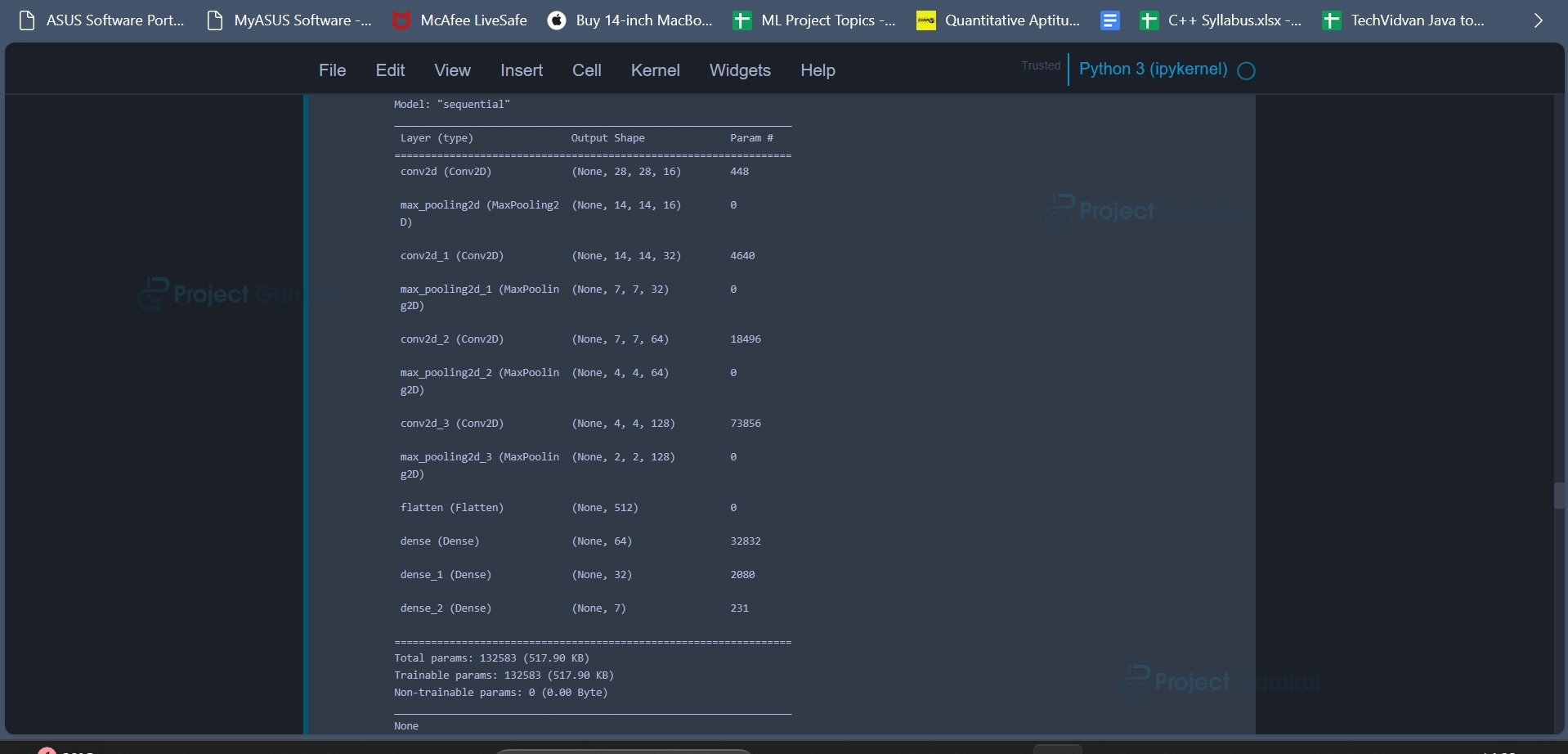
    print(model.summary())
    return model;

Code Explanation:

The code defines a function named create_model that is used to create and configure a convolutional neural network (CNN) model for a multi-class image classification task. The function returns the configured model. This function encapsulates the creation and configuration of a CNN model for image classification and can be used as a building block for further model training and evaluation.

Code:

def train_model(model, X_train, Y_train, EPOCHS=25):
    early_stop = EarlyStopping(monitor='val_loss', patience=10, verbose=1, 
                           mode='auto')
                               #, restore_best_weights=True)
    
    reduce_lr = ReduceLROnPlateau(monitor='val_loss', factor=0.1, patience=3, 
                              verbose=1, mode='auto')
    
    history = model.fit(X_train,
                        Y_train,
                        validation_split=0.2,
                        batch_size = 64,
                        epochs = EPOCHS,
                        callbacks = [reduce_lr, early_stop])
    return history

Code Explanation:

This code defines a function named train_model that is responsible for training a given neural network model with the specified training data. The function takes four arguments:

model: The neural network model to be trained.
X_train: The training features (input data).
Y_train: The corresponding training labels (target values).
EPOCHS (optional): The number of training epochs (default is set to 25).

This function encapsulates the process of training a neural network model with various callbacks to monitor and optimize the training process. It is a convenient way to train models while allowing for customization of training parameters and callbacks.

Code:

def test_model(model, X_test, Y_test):
    model_acc = model.evaluate(X_test, Y_test, verbose=0)[1]
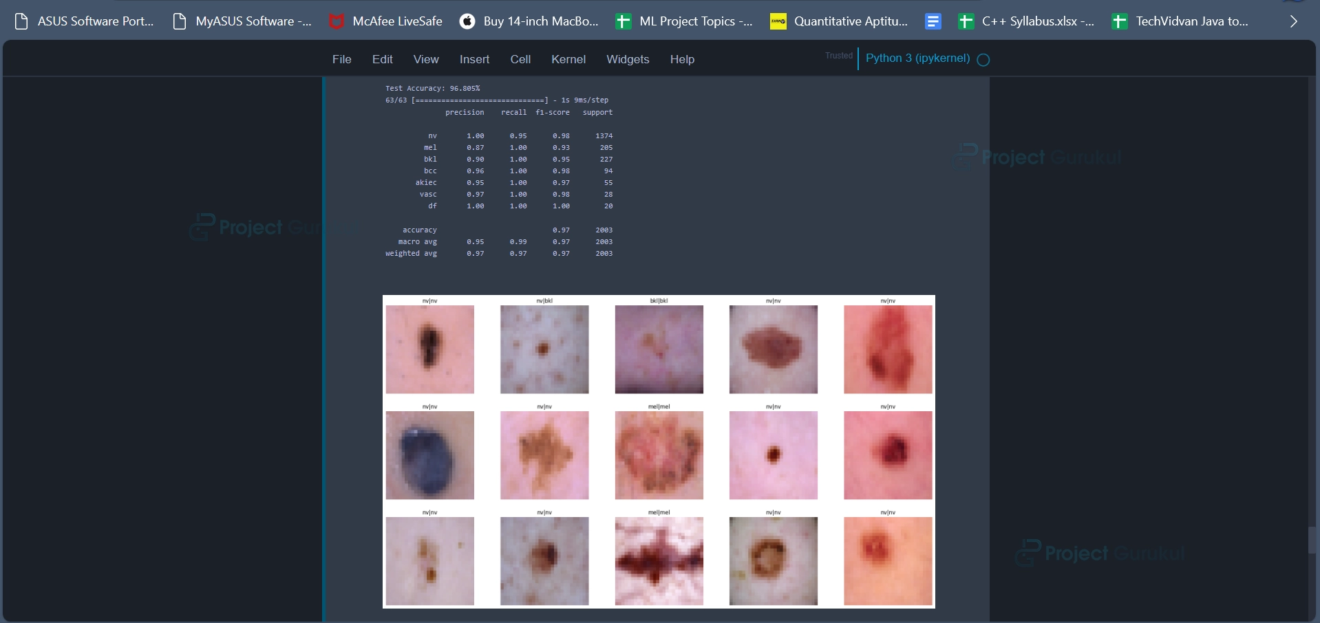
    print("Test Accuracy: {:.3f}%".format(model_acc * 100))
    y_true = np.array(Y_test)
    y_pred = model.predict(X_test)
    y_pred = np.array(list(map(lambda x: np.argmax(x), y_pred)))
    clr = classification_report(y_true, y_pred, target_names=label_mapping.values())
    print(clr)
    
    sample_data = X_test[:15]
    plt.figure(figsize=(22, 12))
    for i in range(15):
        plt.subplot(3, 5, i + 1)
        plt.imshow(sample_data[i])
        plt.title(label_mapping[y_true[i][0]] + '|' + label_mapping[y_pred[i]])
        plt.axis("off")
    plt.show()

Code Explanation:

This code defines a function named test_model that is responsible for evaluating a trained neural network model using a test dataset and displaying various evaluation metrics and visualizations. The function takes three arguments:

model: The trained neural network model to be evaluated.
X_test: The test features (input data).
Y_test: The corresponding test labels (target values).

The model’s accuracy on the test dataset is calculated using the model.evaluate method and the result is stored in the variable model_acc. The accuracy is then printed to the console as a percentage. This function serves as a comprehensive evaluation tool for a classification model, providing insights into accuracy, classification metrics, and visualizations of model predictions on a sample of test data. It aids in assessing the model’s performance and understanding how it performs on specific examples.

Code:

def plot_model_training_curve(history):
    fig = make_subplots(rows=1, cols=2, subplot_titles=['Model Accuracy', 'Model Loss'])
    fig.add_trace(
        go.Scatter(
            y=history.history['accuracy'], 
            name='train_acc'), 
        row=1, col=1)
    fig.add_trace(
        go.Scatter(
            y=history.history['val_accuracy'], 
            name='val_acc'), 
        row=1, col=1)
    fig.add_trace(
        go.Scatter(
            y=history.history['loss'], 
            name='train_loss'), 
        row=1, col=2)
    fig.add_trace(
        go.Scatter(
            y=history.history['val_loss'], 
            name='val_loss'), 
        row=1, col=2)
    fig.show()

Code Explanation:

This code defines a function named plot_model_training_curve that is responsible for creating a visual representation of the training and validation curves of a machine learning model. The function takes a single argument:

history: A history object containing information about the training process, including metrics like accuracy and loss over different epochs. This function is useful for visualizing how a machine learning model’s performance (accuracy and loss) changes during training. It helps in assessing whether the model is converging and whether overfitting or underfitting is occurring.

Code:

def create_confusion_matrix(model, x_test_normalized, y_test, cm_plot_labels, name):
     y_predict_classes, y_true_classes = cal_true_pred_classes(model, x_test_normalized, y_test)
     confusion_matrix_computed = confusion_matrix(y_true_classes, y_predict_classes)
      plot_confusion_matrix(confusion_matrix_computed, cm_plot_labels, name)

Code Explanation:

This code defines a function named create_confusion_matrix that is responsible for creating and plotting a confusion matrix for evaluating the performance of a machine learning model.

The function takes five arguments:

model: The machine learning model to evaluate.
x_test_normalized: The normalized test data (input features).
y_test: The true labels for the test data.
cm_plot_labels: The labels to be used in the confusion matrix plot
name: A name or title for the confusion matrix plot.

This function is a convenient way to generate and visualize a confusion matrix for assessing the classification performance of a machine learning model. It helps in understanding how well the model is performing in terms of correctly and incorrectly classified instances for each class.

Code:

def plot_confusion_matrix(cm, classes,
                          name,
                          normalize=False,
                          title='Confusion matrix',
                          cmap=plt.cm.Blues):
    
    plt.figure(figsize=(8,6))
    plt.imshow(cm, interpolation='nearest', cmap=cmap)
    plt.title(name)
    plt.colorbar()
    tick_marks = np.arange(len(classes))
    plt.xticks(tick_marks, classes, rotation=45)
    plt.yticks(tick_marks, classes)

    if normalize:
        cm = cm.astype('float') / cm.sum(axis=1)[:, np.newaxis]

    thresh = cm.max() / 2.
    for i, j in itertools.product(range(cm.shape[0]), range(cm.shape[1])):
        plt.text(j, i, cm[i, j],
                 horizontalalignment="center",
                 color="white" if cm[i, j] > thresh else "black")
    

    plt.tight_layout()
    plt.ylabel('True Labels')
    plt.xlabel('Predicted Labels')

Code Explanation:

The above code defines a function named plot_confusion_matrix that is responsible for creating and displaying a confusion matrix plot. The function takes several arguments:

cm: The confusion matrix to be plotted.
classes: The class labels used in the confusion matrix.
name: A name or title for the confusion matrix plot.
normalize: A boolean flag that indicates whether the confusion matrix should be normalized or not. If True, the values in the matrix will be divided by the sum of each row to show proportions.
title: The title to be displayed above the confusion matrix plot.
cmap: The colormap to be used for the plot, with a default value of plt.cm.Blues.

This function is used to create a visually informative confusion matrix plot, making it easier to interpret and analyze the classification performance of a machine learning model.

Code:

base_skin_dir = os.path.join('', 'input')

HAM10000_images_part2.zip into one dictionary

imageid_path_dict = {os.path.splitext(os.path.basename(x))[0]: x
                     for x in glob(os.path.join(base_skin_dir,"skin-cancer-mnist-ham10000/", '*', '*.jpg'))}
lesion_type_dict = {
    'nv': 'Melanocytic nevi (nv)',
    'mel': 'Melanoma (mel)',
    'bkl': 'Benign keratosis-like lesions (bkl)',
    'bcc': 'Basal cell carcinoma (bcc)',
    'akiec': 'Actinic keratoses (akiec)',
    'vasc': 'Vascular lesions (vasc)',
    'df': 'Dermatofibroma (df)'
}
label_mapping = {
    0: 'nv',
    1: 'mel',
    2: 'bkl',
    3: 'bcc',
    4: 'akiec',
    5: 'vasc',
    6: 'df'
}
reverse_label_mapping = dict((value, key) for key, value in label_mapping.items())

Code Explanation:

The code begins by defining the base_skin_dir variable, which is a path to a directory containing skin cancer image data. This directory is specified as the input directory. The code’s primary goal is to organize and prepare this image data for further analysis.

Next, the code creates a dictionary called imageid_path_dict. This dictionary is built by iterating through image files in subdirectories of the specified directory. For each image file, the code extracts the image’s filename without its extension and uses it as the key, with the full file path as the corresponding value. Essentially, this dictionary stores the mappings between image IDs and their respective file paths.

This code prepares and organizes skin cancer image data, making it easier to work with and providing essential mappings between image IDs, file paths, lesion types, and their encoded labels.

Code:

data = pd.read_csv(os.path.join(base_skin_dir,"skin-cancer-mnist-ham10000/",'HAM10000_metadata.csv'))

Code Explanation:

In this code, a CSV file containing metadata is read into a Pandas DataFrame. The DataFrame is named data. The data is loaded from a file located in the same directory as the skin cancer image dataset, specifically from the file “HAM10000_metadata.csv”.

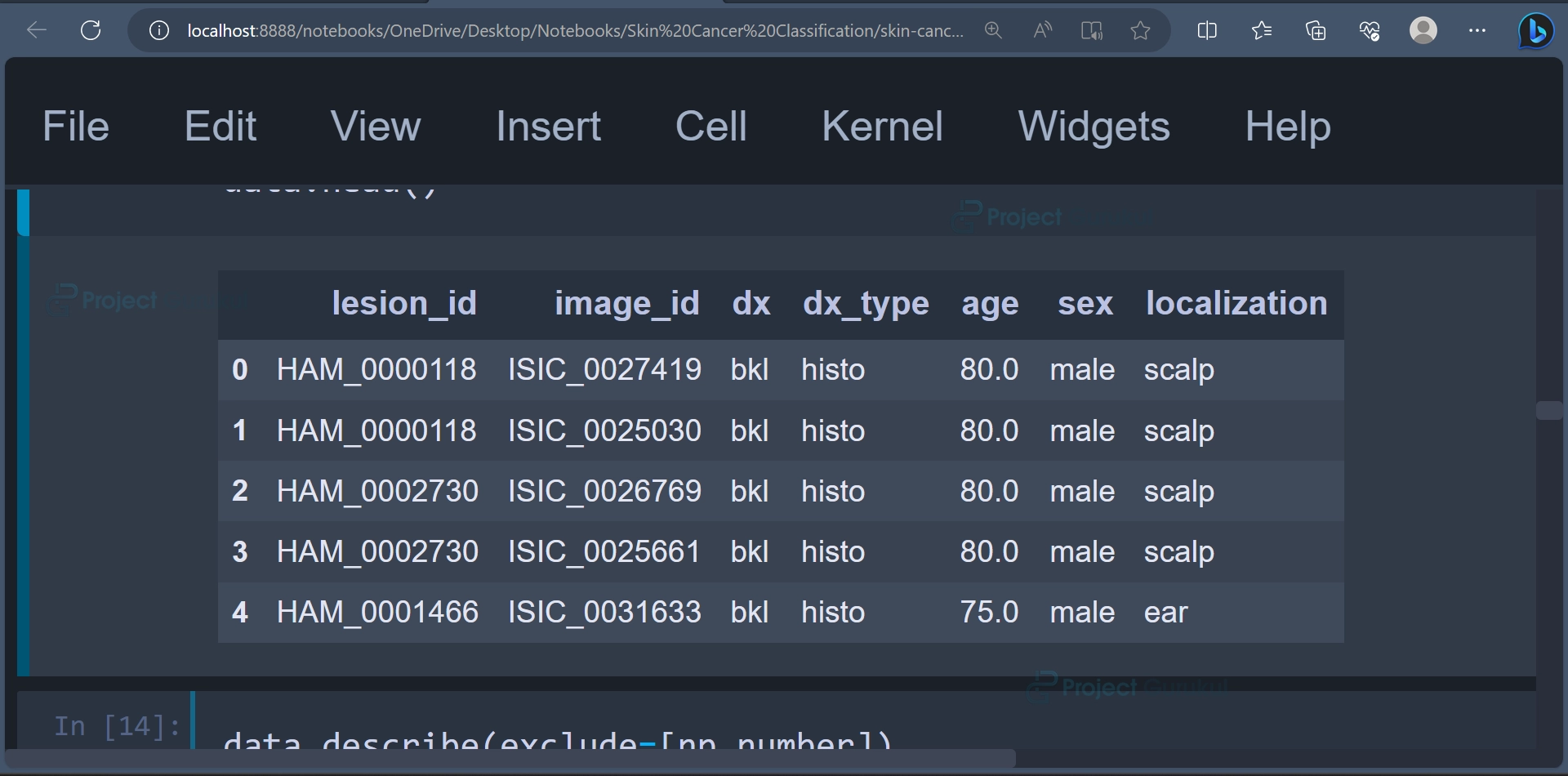
The first few rows of the DataFrame can be displayed using the head() function.

data.head()

Output:

Code:

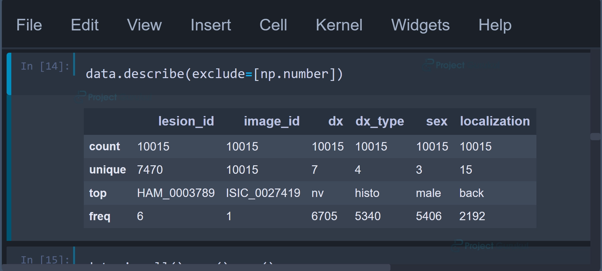
data.describe(exclude=[np.number])

Code Explanation:

The above command is used to generate a summary of statistics for non-numeric (categorical) columns in the Pandas DataFrame named data. This command is typically applied to gain insights into the categorical attributes of the dataset, as it provides statistics specific to these columns.

Output:

Code:

data['age'].fillna(value=int(data['age'].mean()), inplace=True)
data['age'] = data['age'].astype('int32')

Code Explanation:

In this code, the DataFrame is being processed to handle null (missing) values and convert the data type of the ‘age’ column. These operations are common data preprocessing steps to handle missing data and ensure that the data types are appropriate for further analysis or machine learning tasks.

Code:

data['cell_type'] = data['dx'].map(lesion_type_dict.get)
data['path'] = data['image_id'].map(imageid_path_dict.get)

Code Explanation:

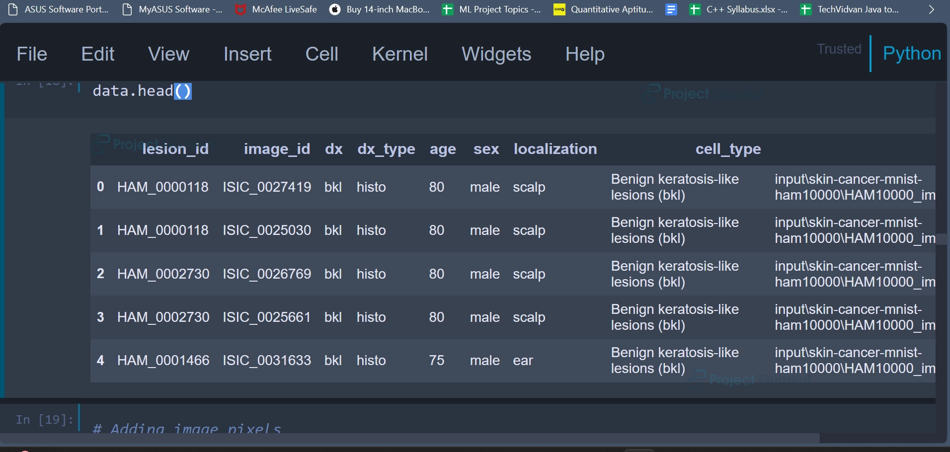
Using this code we are adding two new columns, ‘cell_type’ and ‘path,’ that are added to the DataFrame. The first line of code creates a new column ‘cell_type’ in the DataFrame. It maps the values in the ‘dx’ column to their corresponding descriptions using the lesion_type_dict dictionary. By using the map function with lesion_type_dict.get, it replaces the abbreviations with their descriptive names.

The second line of code creates another new column ‘path’ in the DataFrame. It maps the values in the ‘image_id’ column to their corresponding file paths using the imageid_path_dict dictionary. The ‘image_id’ column contains unique identifiers for images, and imageid_path_dict maps these identifiers to the actual file paths of the images.

Once these operations are done, the first 5 rows of the DataFrame can be displayed using the first head() function.

data.head()

Output:

Code:

data['image_pixel'] = data['path'].map(lambda x: np.asarray(Image.open(x).resize((28,28))))

Code Explanation:

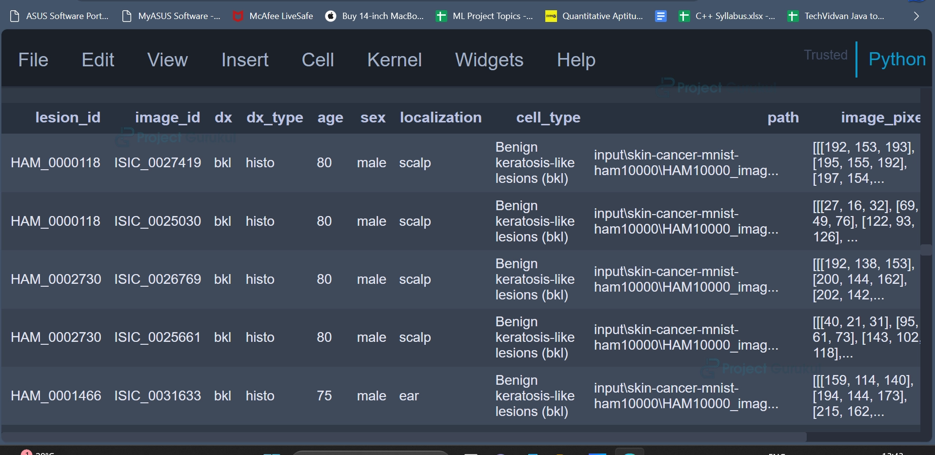
In this line of code, a new column ‘image_pixel’ is created in the DataFrame data. This column contains the pixel data of the images represented as NumPy arrays. The ‘image_pixel’ column will contain NumPy arrays, where each array represents the pixel values of a resized image. These pixel values can be used as input data for training machine learning models or deep learning models.

The first 5 rows of the DataFrame can be displayed again in a similar fashion.

data.head(5)

Output:

Code:

sample_data = data.groupby('dx').apply(lambda df: df.iloc[:2, [9, 7]])
plt.figure(figsize=(22, 32))
for i in range(14):
    plt.subplot(7, 5, i + 1)
    plt.imshow(np.squeeze(sample_data['image_pixel'][i]))
    img_label = sample_data['cell_type'][i]
    plt.title(img_label)
    plt.axis("off")
plt.show();

Code Explanation:

In this code snippet, a sample of images from the dataset is selected and displayed using Python’s Matplotlib library. The purpose of this code is to visualize a subset of the skin lesion images along with their corresponding labels. The first line of code groups the data by the ‘dx’ column, which represents the diagnosis labels for different skin lesions. For each group (skin lesion type), it selects the first two rows of data and specifically extracts columns at indices 9 and 7. These columns correspond to ‘image_pixel’ (containing image pixel data) and ‘cell_type’ (representing the cell type or skin lesion label), respectively.

plt.imshow(np.squeeze(sample_data[‘image_pixel’][i])) displays the image data from the ‘image_pixel’ column of ‘sample_data.’ The np.squeeze() function is used to remove any single-dimensional entries from the shape of the image array, ensuring it is a valid image for display.

Overall, this code provides a visual representation of a subset of skin lesion images, making it easier to understand and inspect the dataset.

Output:

Code:

data['label'] = data['dx'].map(reverse_label_mapping.get)
data = data.sort_values('label')
data = data.reset_index()

Code Explanation:

In the above code, additional data processing steps are performed on the skin cancer dataset. These steps involve mapping the diagnosis labels to numerical values and sorting the data based on these labels. They convert diagnosis labels into numerical values, sort the data by these labels, and reset the DataFrame index for further analysis and model training. These steps are essential for preparing the dataset for tasks like classification.

Code:

counter = 0
frames = [data]
for i in [4,4,11,17,45,52]:
    counter+=1
    index = data[data['label'] == counter].index.values
    df_index = data.iloc[int(min(index)):int(max(index)+1)]
    df_index = df_index.append([df_index]*i, ignore_index = True)
    frames.append(df_index)

Code Explanation:

This code performs data augmentation by replicating rows for specific classes or categories within a dataset multiple times. The augmentation factors for each class are specified in the list [4, 4, 11, 17, 45, 52]. This technique is commonly used to increase the diversity of training data, which can improve the performance of machine learning/deep learning models when dealing with imbalanced datasets or when additional training samples are needed.

final_data = pd.concat(frames)

The above code snippet combines and concatenates multiple DataFrames stored in the ‘frames’ list into a single DataFrame named ‘final_data’.

Code:

X_orig = data['image_pixel'].to_numpy()
X_orig = np.stack(X_orig, axis=0)
Y_orig = np.array(data.iloc[:, -1:])

Code Explanation:

In this code snippet:

‘X_orig’ is created as a NumPy array. This variable will store the image data for the machine learning task. Initially, it is assigned the pixel data of the images from the ‘image_pixel’ column.
‘np.stack(X_orig, axis=0)’ is used to stack the image arrays along the first axis (axis=0), effectively creating a 4D array where each element represents an image.
‘Y_orig‘ is created as a NumPy array. This variable will store the corresponding labels or target values for the machine learning/deep learning task. It is assigned the values from the last column (‘label’).

The same code can be used again for the augmented data as well.

X_aug = final_data['image_pixel'].to_numpy()
X_aug = np.stack(X_aug, axis=0)
Y_aug = np.array(final_data.iloc[:, -1:])

‘X_aug’ contains the augmented image data, and ‘Y_aug’ contains the corresponding labels or target values. These arrays are prepared for training and evaluating machine learning models, particularly deep learning models for image classification, using the augmented dataset. Augmentation is a common technique to increase the diversity of training data and improve model performance.

Code:

X_train_orig, X_test_orig, Y_train_orig, Y_test_orig = prepare_for_train_test(X_orig, Y_orig)

Code Explanation:

The code is splitting the original image and label data into training and testing sets using a predefined function called prepare_for_train_test.

Code:

model =create_model()

Code Explanation:

The code is creating a machine learning or deep learning model using a function called create_model.

Output:

Code:

X_train_aug, X_test_aug, Y_train_aug, Y_test_aug = prepare_for_train_test(X_aug, Y_aug)

Code Explanation:

Similar to splitting the original data into training sets and testing sets, we can also split the augmented image data into training sets and testing sets, using the prepare_for_train_test function.

Code:

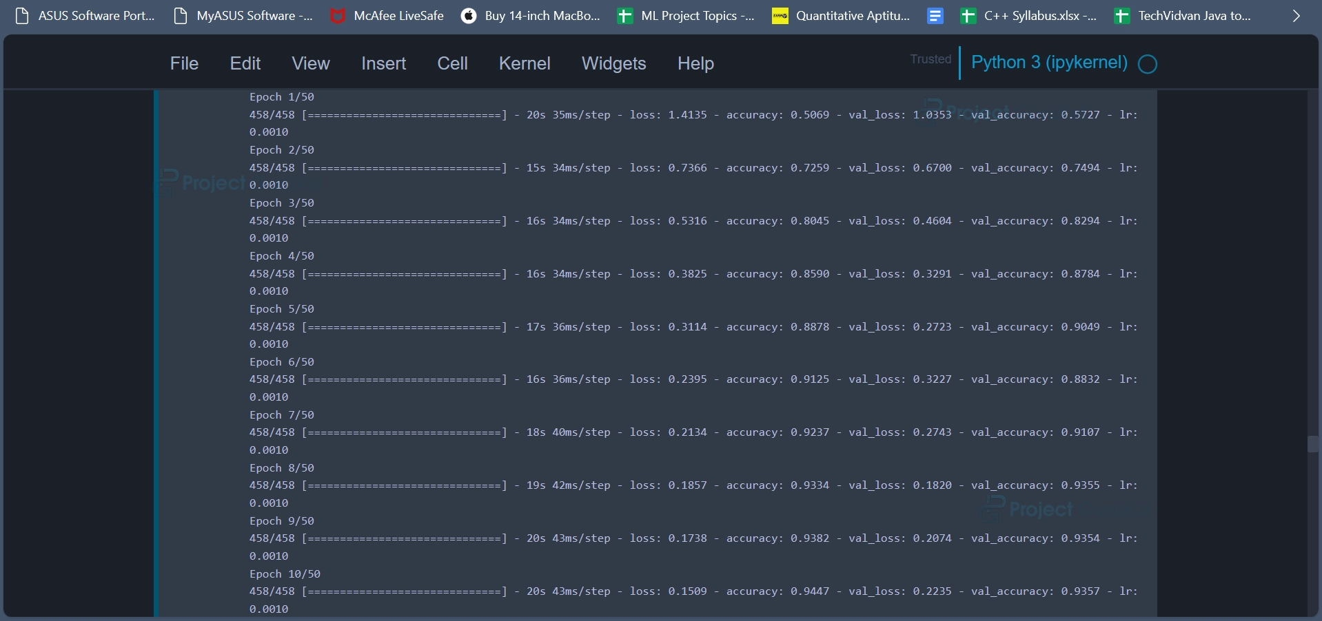
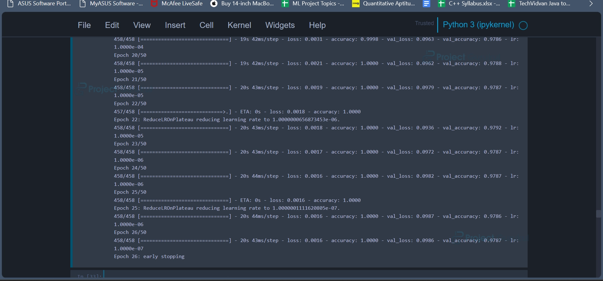
model2_history = train_model(model, X_train_aug, Y_train_aug, 50)

Code Explanation:

The objective of the code snippet is to train the previously created deep learning model (model) using augmented data. This code trains a deep learning model on augmented training data with the specified number of epochs while monitoring the validation loss. Early stopping and learning rate reduction are used to prevent overfitting and improve training efficiency. The training progress and performance metrics are stored in model2_history for later analysis and visualization.

Output:

Code:

model.save('Skin_Cancer.sav')

Code Explanation:

The above code saves the trained deep learning model to a file named “Skin_Cancer.sav.” This is a common practice in machine learning and deep learning to save models after training so that they can be reused later without having to retrain them from scratch.

model.save_weights("Skin_Cancer.hdf5")

The above code saves only the weights of the trained deep learning model to a file named “Skin_Cancer.hdf5.” Unlike saving the entire model (as done previously), this approach saves only the model’s weights, excluding the model architecture and other information.

Code:

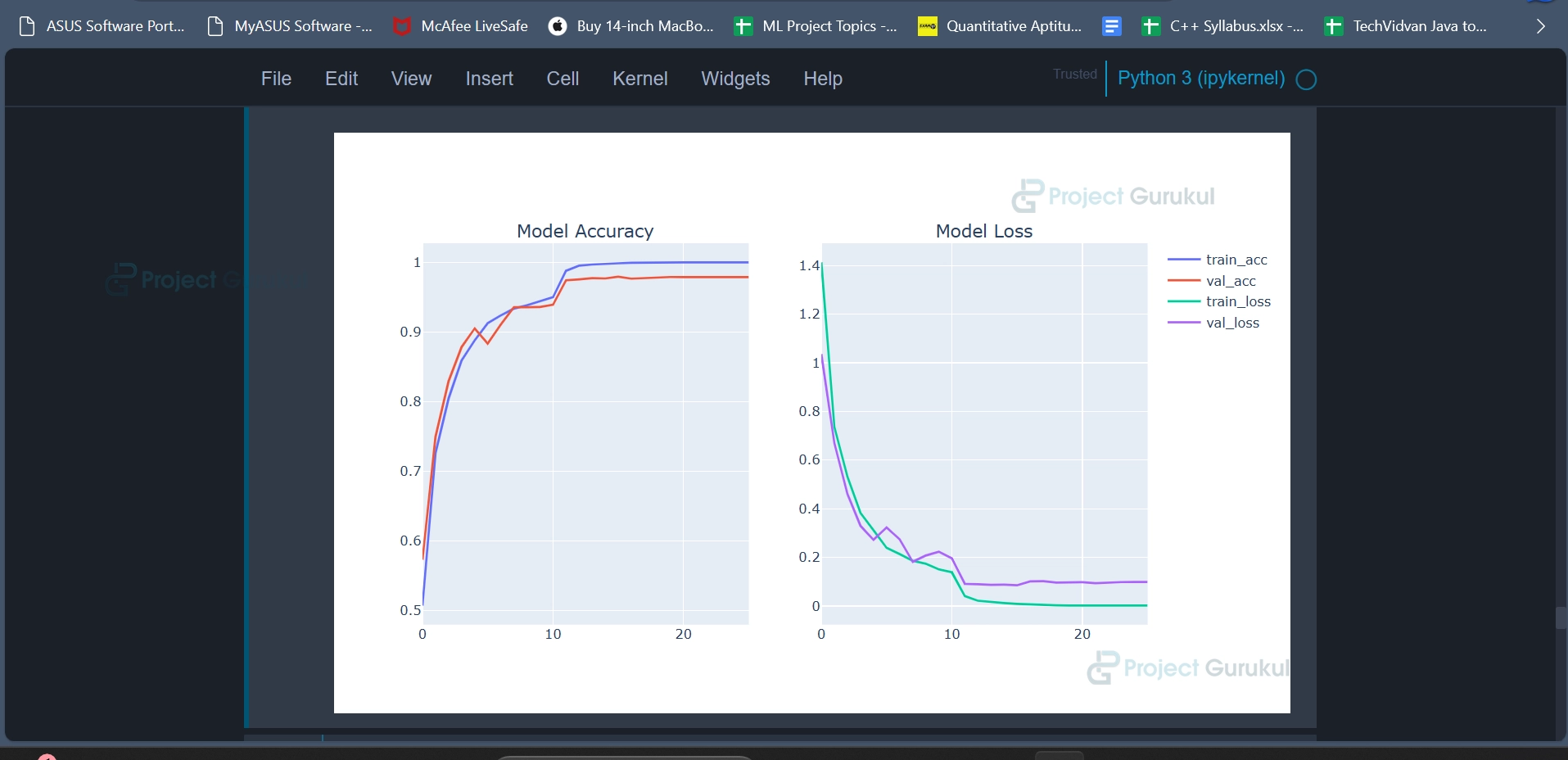
plot_model_training_curve(model2_history)

Code Explanation:

The code snippet is used to visualize the training and validation performance of a deep learning model during training. It plots two key metrics, accuracy, and loss, over the training epochs to help assess the model’s performance. This function helps us monitor and analyze the training progress of the deep learning model.

Output:

Code:

test_model(model, X_test_orig, Y_test_orig)

Code Explanation:

The test_model function is used to evaluate a deep learning model’s performance on a test dataset and provide various evaluation metrics and visualizations. It reports accuracy, classification metrics etc to help users gauge the model’s effectiveness in skin cancer classification.

Output:

Code:

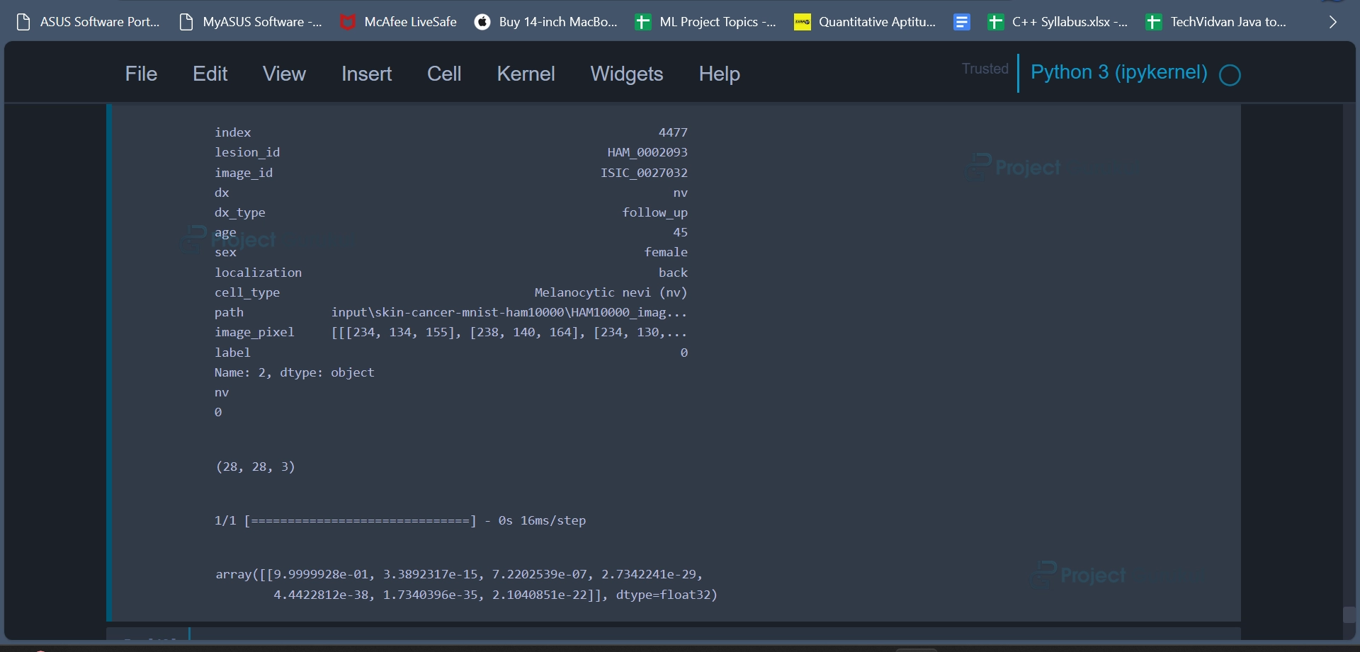
one_picture_predict_data = data.iloc[2]
print(one_picture_predict_data)
print(one_picture_predict_data.dx)
y_value = reverse_label_mapping.get(one_picture_predict_data.dx)
print(y_value)


one_picture_predict_data.image_pixel.shape
new_one = one_picture_predict_data.image_pixel.reshape((1,28,28,3))
model.predict(new_one)

Code Explanation:

This code snippet is designed to predict the class label of a single skin cancer image (random image from dataset) based on its pixel data using a pre-trained deep learning model. It involves extracting information from the dataset, converting labels, reshaping the image, and ultimately obtaining the model’s prediction for the image’s class.

Output:

Code:

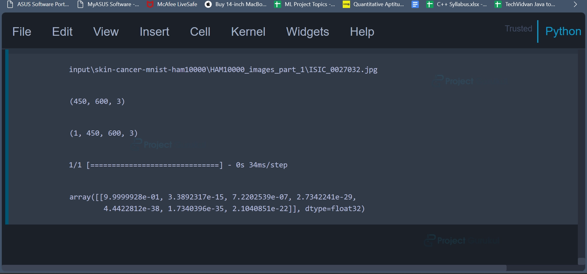
print(data.iloc[2].path)
im = np.asarray(Image.open(data.iloc[2].path))
im.shape
im = im.reshape((1,450,600,3))
im.shape
new_one = one_picture_predict_data.image_pixel.reshape((1,28,28,3))
model.predict(new_one)

Code Explanation:

This code snippet showcases image loading, reshaping, and prediction processes. It demonstrates how to prepare an image for classification using a deep learning model by adjusting its dimensions to match the model’s input shape and then obtaining a prediction based on the modified image.

Output:

Conclusion

In conclusion, the Machine Learning Skin Cancer Classification project successfully demonstrated the effectiveness of deep learning techniques in diagnosing skin lesions. It showcased the importance of data preprocessing, augmentation, and model tuning in achieving accurate and reliable results. This project’s outcomes have the potential to assist medical professionals in the early detection and diagnosis of various skin conditions, ultimately contributing to better patient care and outcomes.