Machine Learning Project – Predicting Diabetes

Diabetes can be defined as a long-lasting condition where the process of conversion of food to energy is affected, leading to an imbalance in the blood sugar levels in the body. It is caused by either the pancreas not making enough insulin or the body not adequately using the insulin produced. Insulin is a hormone that regulates the quantity of sugar in the blood.

Diabetes symptoms include frequent urination, excessive thirst, hunger, weariness, impaired eyesight, and poor wound healing. Diabetes, if not controlled, can cause major consequences such as heart disease, renal disease, nerve damage, and blindness. Diabetes is often diagnosed by blood sugar level testing. Diabetes treatment often consists of medicine, lifestyle adjustments such as diet and exercise, and blood sugar monitoring.

Machine learning algorithms may be used to analyse enormous volumes of data to detect trends and anticipate diabetic outcomes. This can assist healthcare providers in making better-informed decisions about illness diagnosis, treatment, and management.

Dataset

The dataset used in this project is a popular dataset used in various machine-learning projects for the prediction of diabetes.

The dataset contains 768 instances, each with eight attributes and one target variable. The attributes include skin thickness ( skin fold thickness), Glucose (Plasma glucose concentration), Age (in years) etc.

The target variable is a binary variable indicating whether or not the patient has diabetes. There are two kinds of values present in the target variable (Outcome), which indicate whether a person has diabetes or not.

The dataset can be downloaded from this link.

Tools and Libraries Used

The project makes use of the following Python libraries:
· NumPy
· Pandas
· Matplotlib
· Seaborn
· Scikit-Learn

Download Machine Learning Predicting Diabetes Project

Please download the source code of Machine Learning Predicting Diabetes Project from the following link: Machine Learning Predicting Diabetes Project Code

Steps for Predicting Diabetes Using Machine Learning

1. Importing the required libraries.

import pandas as pd
import numpy as np
import matplotlib.pyplot as plt
import seaborn as sns

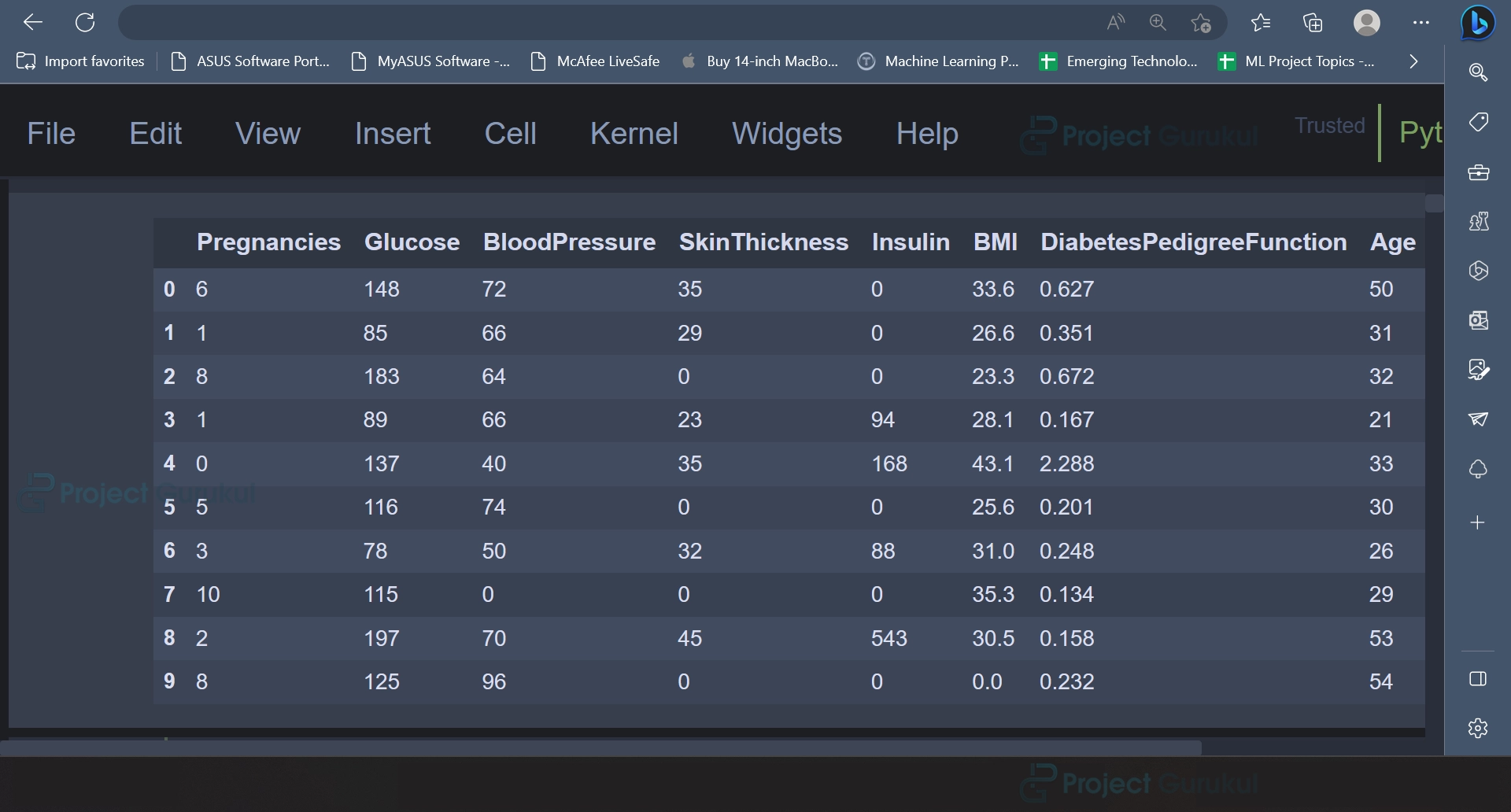
2. After importing the necessary libraries, the dataset can be read using the read_csv() function. The first 10 rows have been displayed in the screenshot shown below. The dataset contains features like blood pressure, body mass index (BMI), age, etc.

data = pd.read_csv('diabetes_data.csv')
# Display the first 10 rows of data
data.head(10)

Output:
In the below output, the first ten rows of the dataset have been displayed.

3. Exploratory data analysis, also known as EDA, is a significant method to gain insights from the data. It is evident that the dataset contains 768 rows and nine columns.

data.info()

Output
To know more about the dataset, the info() function can be used. The output contains information regarding factors like the number of rows and columns present in the dataset and the data type of all the columns in the dataset.

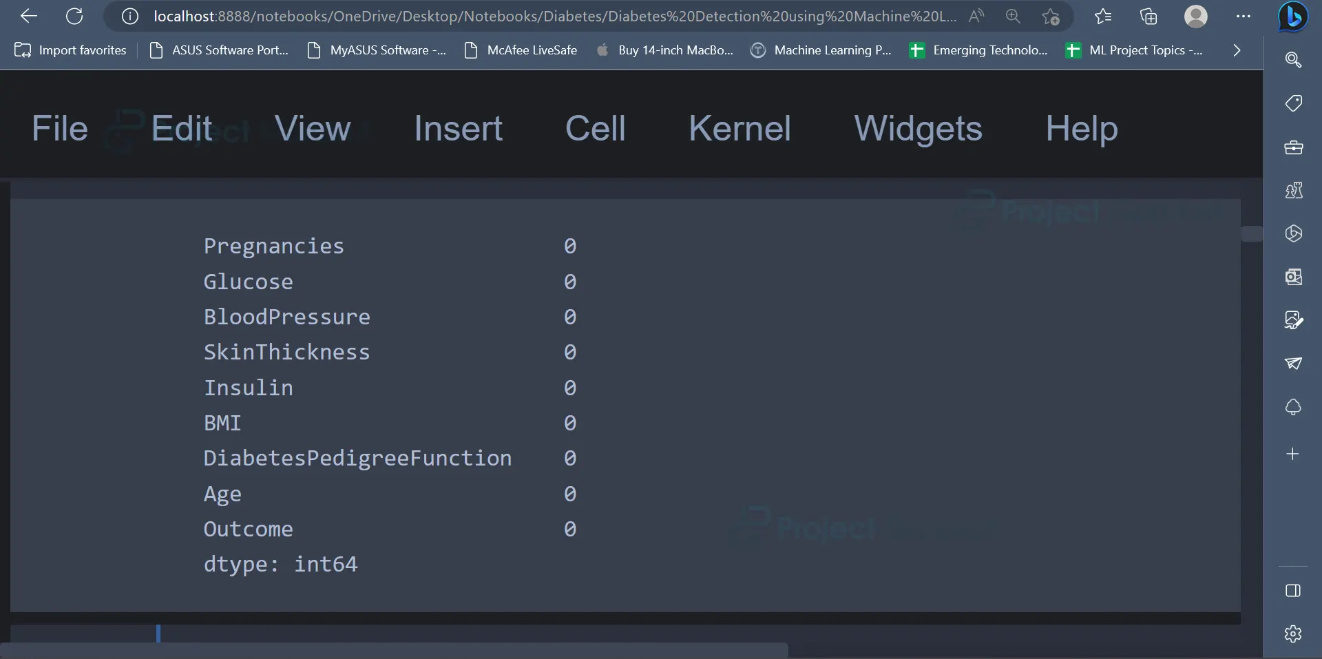
4. Some datasets usually contain some missing values or null values. These values have to be handled accordingly before we train machine learning models using this data. The below code gives the number of null values present in each column.

data.isnull().sum()

Output
The output indicates the number of null values present in each column of the dataset. From the output it is clear that there are no null values present in the dataset.

5. The describe() function can be used to get a statistical summary of the data such as mean, min, max, standard deviation, etc.

data.describe()

Output
The output indicates the count, mean, standard deviation, minimum, and maximum values for all the attributes of the dataset.

6. After gaining some statistical information about the dataset, the data can be represented in a graphical or visual format such as charts, graphs, maps, and infographics to help understand and analyse it. It is a powerful tool for data exploration, communication, and storytelling.

plt.style.use('ggplot')
plt.figure(figsize=(10, 5))
plt.title('Glucose Distribution')
sns.distplot(data['Glucose'])
plt.show()

Output
The data present in the glucose column is displayed using a histogram in the output. The data is normally distributed since the histogram is a bell-shaped curve.

The above code uses a histogram to plot the Glucose attribute present in the dataset. A good way to represent numerical data would be using a histogram. It is a way of summarising the frequency of observations in a set of continuous or discrete data.

7. The same code can be used to plot the histogram for other attributes as well.

plt.style.use('ggplot')
plt.figure(figsize=(10, 5))
plt.title('BloodPressure Distribution')
sns.distplot(data['BloodPressure'])
plt.show()

Output

plt.style.use('ggplot')
plt.figure(figsize=(10, 5))
plt.title('BMI Distribution')
sns.distplot(data['BMI'])
plt.show()

Output

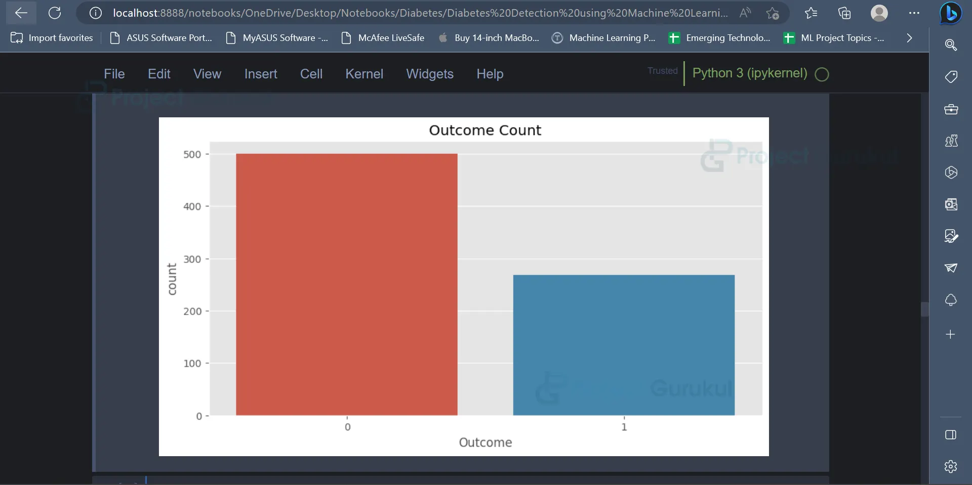
8. The outcome column indicates whether a person has diabetes or not. The distribution of the values present in the outcome column can be visually represented using a countplot.

plt.figure(figsize=(10, 5))
sns.countplot(data['Outcome'])
plt.title('Outcome Count')
plt.show()

Output
In the below image, the distribution of the values present in the outcome column can be observed.
The value 0 has a count of 500, and the value 1 has a count of 268 in the outcome column.

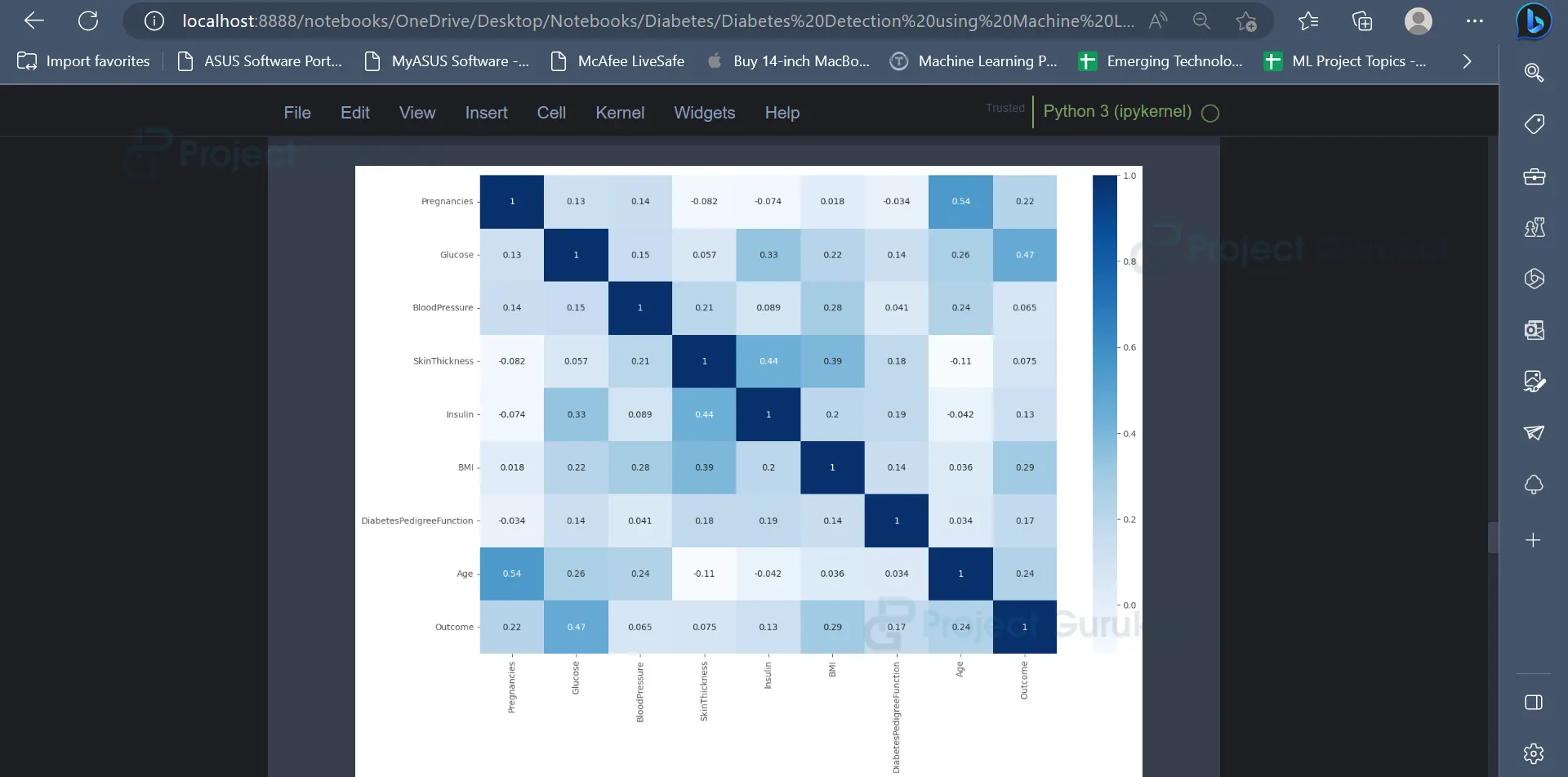
9. A correlation matrix can be used to understand the relationship between various variables present in the dataset, as well as how every variable affects every other variable present in the dataset.

corr = data.corr()
corr['Outcome'].sort_values(ascending=False)
plt.figure(figsize=(15, 10))
sns.heatmap(corr, annot=True, cmap='Blues')
plt.show()

Output
A correlation matrix indicating the relationship between the various features of the dataset is displayed below.

10. Now that the data has been represented using graphs and charts, some data preprocessing can be carried out. This step involves transforming the raw data into a format which is more suitable for further analysis.

from sklearn.preprocessing import StandardScaler
scale = StandardScaler()
newData = pd.DataFrame(scale.fit_transform(data), columns=data.columns)

This method can be used to scale the attributes of the dataset. Initially, an instance of the StandardScaler is created. Then, the fit_transform method is used to apply the scaling to the dataframe called data and create a new dataframe called newData. The columns=data.columns are used so that the new dataframe (newData) has the same column names as the original dataframe (data).

11. Now, the data can be split into training data and testing data. Using the training data, we can train machine learning models, and the accuracy of these models can be tested using the testing dataset.

from sklearn.model_selection import train_test_split
xtrain, xtest, ytrain, ytest = train_test_split(newData, target, test_size=0.2, random_state=42)

12. As mentioned earlier, we use the training dataset in the next step to train multiple machine-learning models. Models like Random Forest Classifiers and Support Vector Machines can be trained using the training dataset.

from sklearn.svm import SVC
svc = SVC()
param = {
    'C': [i for i in range(1, 10)],
    'kernel': ['rbf', 'linear', 'poly']}

grid = GridSearchCV(svc, param, cv=5, scoring='neg_mean_squared_error')
grid.fit(xtrain, ytrain)

SvcModel = grid.best_estimator_
SvcModel.fit(xtrain, ytrain)

svc_pred = SvcModel.predict(xtest)

Grid Search CV is a machine learning approach for determining the best hyperparameters for a given model. Hyperparameters, such as learning rate, regularisation strength, and number of hidden layers, are not learnt from data but are specified before training the model. The performance of the model is affected by the value of the hyperparameters.

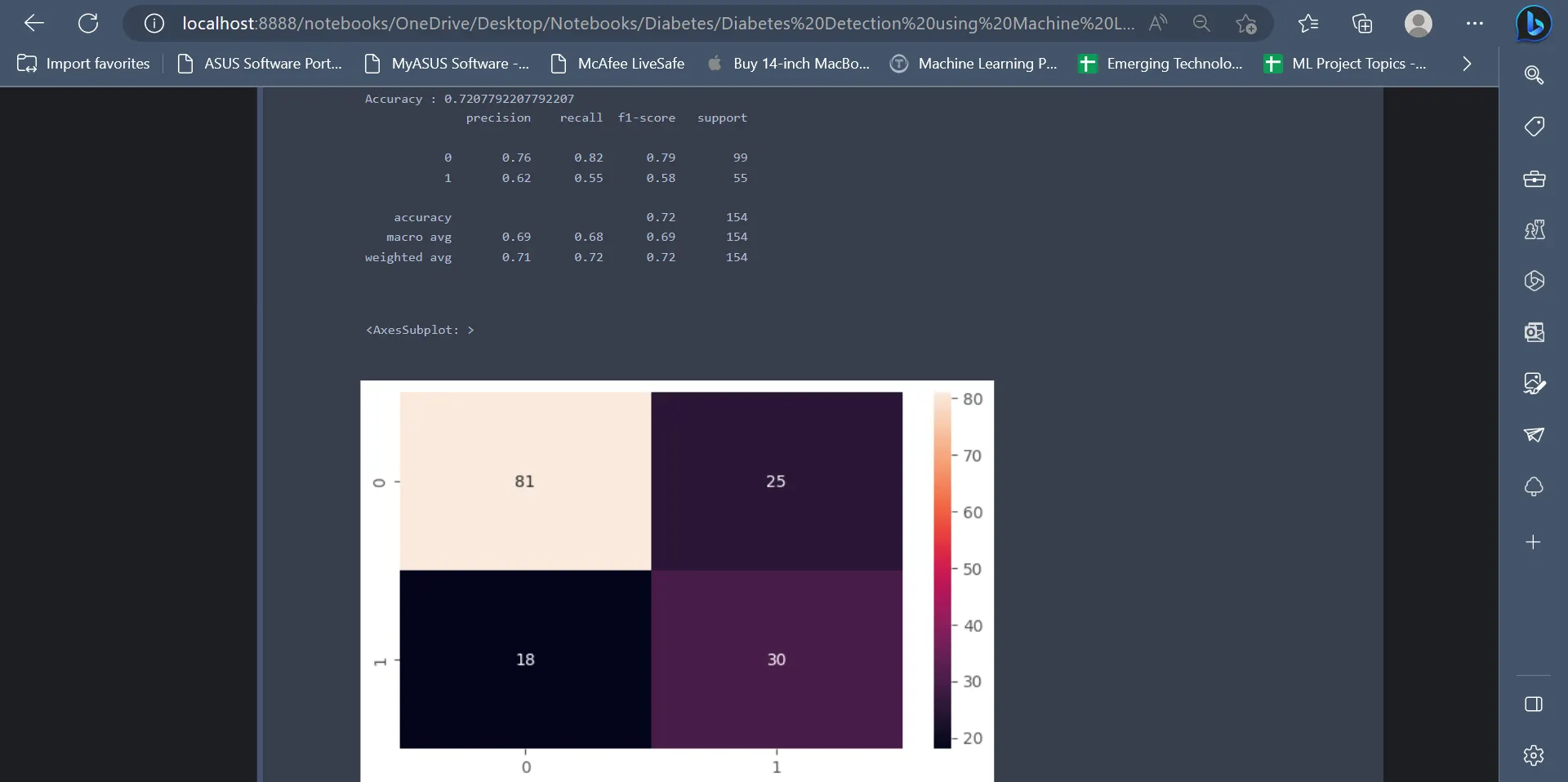
From the below code, it is evident that the Support Vector Classifier has an accuracy of 72.07%. The classification report gives insights regarding precision, f1-score, recall, etc.

print("Accuracy :",accuracy_score(ytest, svc_pred))
print(classification_report(ytest, svc_pred))
plt.figure(figsize = (7,4))
sns.heatmap(confusion_matrix(svc_pred,ytest), annot = True)

Output
The output displays metrics like classification reports, accuracy scores, and confusion matrix for the SVC classifier.

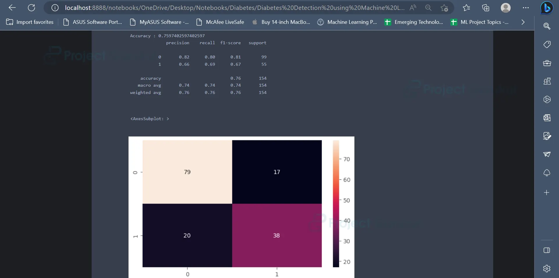
13. The next model which we will be using is the Random Forest Classifier. Random Forest Classifier has an accuracy of 75.97% on the dataset.

from sklearn.ensemble import RandomForestClassifier
random = RandomForestClassifier()
parameters = {
    'n_estimators': [100, 200, 300, 400, 500, 600],
    'criterion': ['gini', 'entropy']}
    
gridSearch = GridSearchCV(random, parameters, cv=5, scoring='neg_mean_squared_error')
gridSearch.fit(xtrain, ytrain)

RandomForestModel = gridSearch.best_estimator_
RandomForestModel.fit(xtrain, ytrain)

rf_pred = RandomForestModel.predict(xtest)


print("Accuracy :",accuracy_score(ytest, rf_pred))
print(classification_report(ytest, rf_pred))
plt.figure(figsize = (7,4))
sns.heatmap(confusion_matrix(rf_pred,ytest), annot = True)

Output
The output displays metrics like classification report, accuracy score, and confusion matrix for Random Forest Classifier.

14. The last algorithm which we will be using is the Gradient Boosting Classifier. The Gradient Boosting Classifier has an accuracy of 74.67% on the dataset.

from sklearn.ensemble import GradientBoostingClassifier
GradientModel = GradientBoostingClassifier()
GradientModel.fit(xtrain, ytrain)
gradient_pred = GradientModel.predict(xtest)


print("Accuracy :",accuracy_score(ytest, gradient_pred))
print(classification_report(ytest, gradient_pred))
plt.figure(figsize = (7,4))
sns.heatmap(confusion_matrix(gradient_pred,ytest), annot = True)

Output
The next output displays metrics like classification report, accuracy score, and confusion matrix for the Gradient Boosting algorithm.

Conclusion

To summarise, diabetes is a significant and widespread health problem that affects millions of individuals globally. Machine learning has shown considerable promise in the early identification and diagnosis of diabetes, which can assist in improving patient outcomes and saving healthcare costs.

Overall, the use of machine learning in diabetes detection and treatment is a promising area of research that has the potential to revolutionise healthcare. With further advancement in technology and research, these Machine Learning models will be able to train on much larger datasets, which would eventually result in much better predictions and improved accuracy.