Machine Learning Project – Earthquake Prediction

What is an Earthquake?

Earthquakes are something which almost everyone has heard about or experienced at some point or other. Earthquakes are basically naturally occurring event which occurs when there is a sudden release of energy in the Earth’s crust resulting in vibrations or shaking of the ground. Under the surface of the earth, there are large sections called tectonic plates which make up the outer layer of the earth. These sections are frequently moving and interact with each other. As a result of this interaction and movement, these plates can get locked due to friction, which in turn causes stress to build up. Over time, as the stress keeps accumulating, at one point, it reaches a point at which the rocks along the boundaries of the plates rupture, releasing a vast amount of stored energy. This energy, which is released, propagates as Seismic waves through the earth’s crust, thus causing the ground to shake and tremble. The strength as well as intensity of an earthquake is measured using a standard scale known as the Richter scale.

Dataset

The earthquake dataset contains detailed information regarding the various earthquakes which have happened around the world between 1-01-2001 and 1-01-2023. It is structured data related to Seismic events. Such data is collected and maintained by organisations like seismological institutes, research institutes etc. This dataset can be used to build and train various Machine Learning models which can predict earthquakes which would help in saving people’s lives and also to take necessary measures to reduce the damage caused.

The dataset contains 782 rows and 19 attributes (columns) in total. A brief description of the attributes are:

title: Refers to the name/title given to the earthquake

magnitude: Used to describe the strength or intensity of the earthquake

date_time: Indicates the date and time of the earthquake

CDI: CDI represents the highest level of reported intensity recorded for the given earthquake

MMI: MMI stands for Modified Mercalli Intensity and indicates the maximum reported instrumental intensity for the earthquake

alert: This attribute refers to the alert level, which indicates the possible threat or risk associated with a particular earthquake

tsunami: Indicates whether the earthquake caused a tsunami or not

sig: Used to describe how significant an earthquake is. The significance of the earthquake is directly proportional to this number

net: Indicates the id of the source which collected the data.

nst: This attribute is used to describe the overall count of seismic stations utilised for establishing the location of the earthquake.

dmin: Indicates the closest station’s horizontal distance from the epicentre.

gap: Used to determine the horizontal position of the earthquake. A smaller value indicates greater reliability in determining the horizontal position of the earthquake

magType: This refers to the type of algorithm used to calculate the magnitude of an earthquake

depth: Indicates the depth at which the earthquake begins to rupture

latitude, longitude: Indicates the location of the earthquake using a coordinate system

location: Indicates the specific location within the country

continent: Refers to the continent where the earthquake occurred

country: Indicates the country affected by the earthquake

Tools and Libraries Used

The project makes use of the following Python libraries:

• NumPy
• Matplotlib
• Seaborn
• Pandas
• Scikit-Learn

Prerequisites For Earthquake Prediction Using Machine Learning

The prerequisites required are:

NumPy

• Understanding of arrays and matrix operations.
• Ability to perform numerical computations efficiently

Pandas

• Proficiency in handling and analysing structured data.
• Understanding of DataFrames and Series.
• Ability to manipulate and preprocess seismic data, including cleaning, filtering, and transforming data.

Matplotlib

• Knowledge of basic plotting techniques, including line plots, scatter plots, and histograms.
• Understanding of subplots for creating multiple plots in a single figure.
• Familiarity with advanced plot types, such as heat maps, contour plots, and geographical visualisations.

Seaborn

• Understanding of statistical data visualisation techniques.
• Knowledge of Seaborn functions for creating visually appealing and informative plots.

scikit-learn

• Familiarity with machine learning concepts, such as supervised and unsupervised learning.
• Understanding of model selection, training, and evaluation procedures.

Download Machine Learning Earthquake Prediction Project

Please download the source code of Machine Learning Earthquake Prediction Project: Machine Learning Earthquake Prediction Project Code

Steps for Earthquake Detection Using Machine Learning

1. Importing the required libraries.

import pandas as pd
import numpy as np
import matplotlib.pyplot as plt
import seaborn as sns

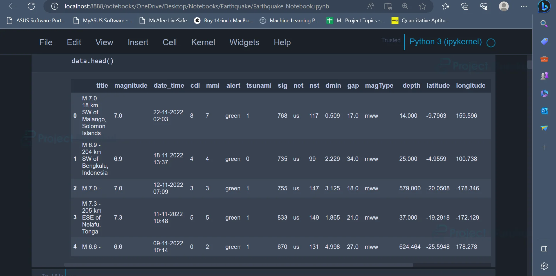
2. After importing the required libraries, the dataset can be read and displayed. The dataset can be read using the read_csv() function, and the first five rows of the dataset can be displayed using the head() function.

data = pd.read_csv('earthquake_data.csv')
data.head()

Output

The output displays the first five rows of the dataset.

3. Once the data has been read, some basic exploratory data analysis can be carried out on the data in order to gain some insights about the data and to understand more about the data.

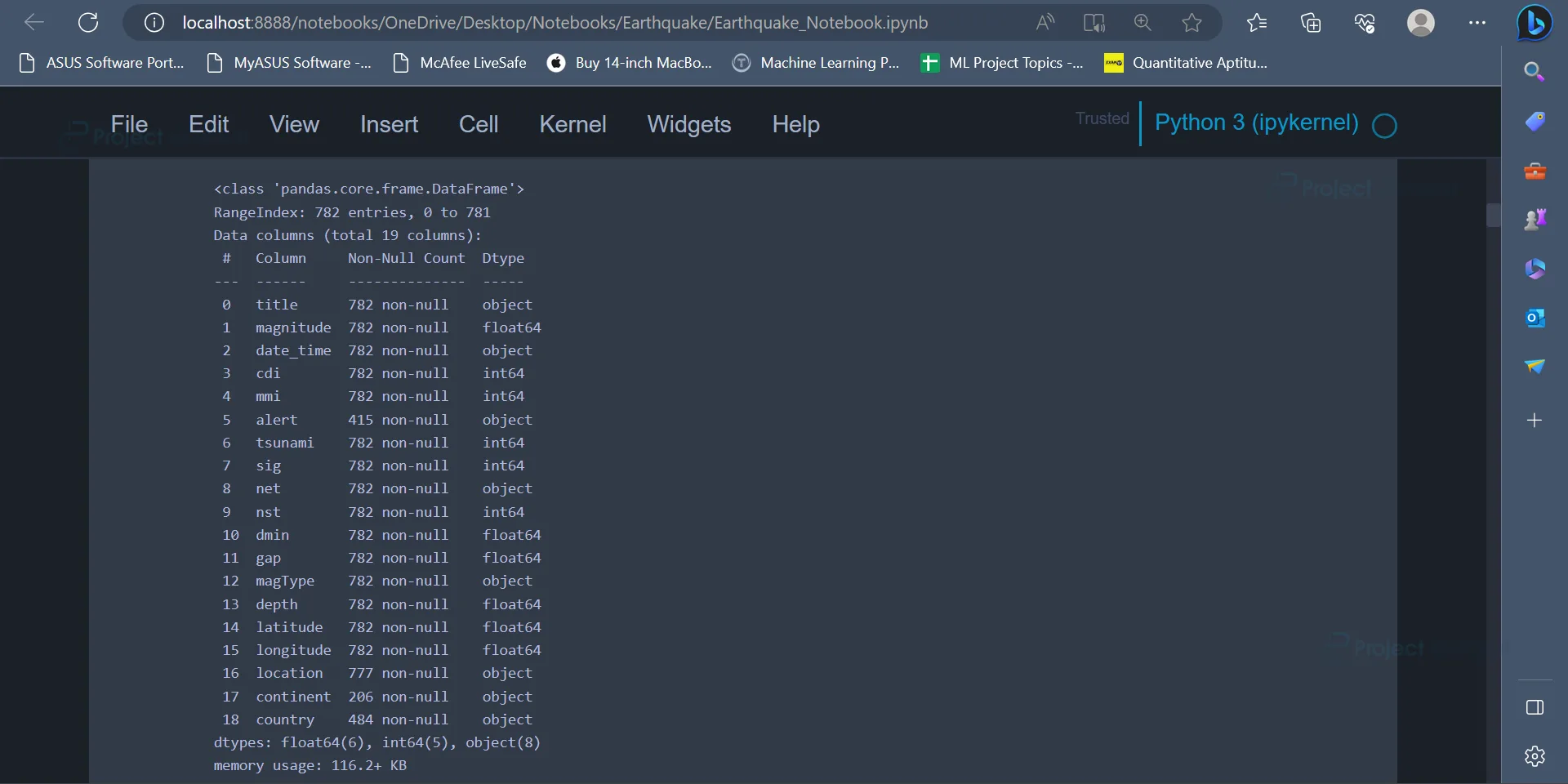
data.info()

Output

The info() function is used to get information regarding the attributes present in the dataset, the number of rows in the dataset, the number of missing values in each attribute, the data type of each attribute etc.

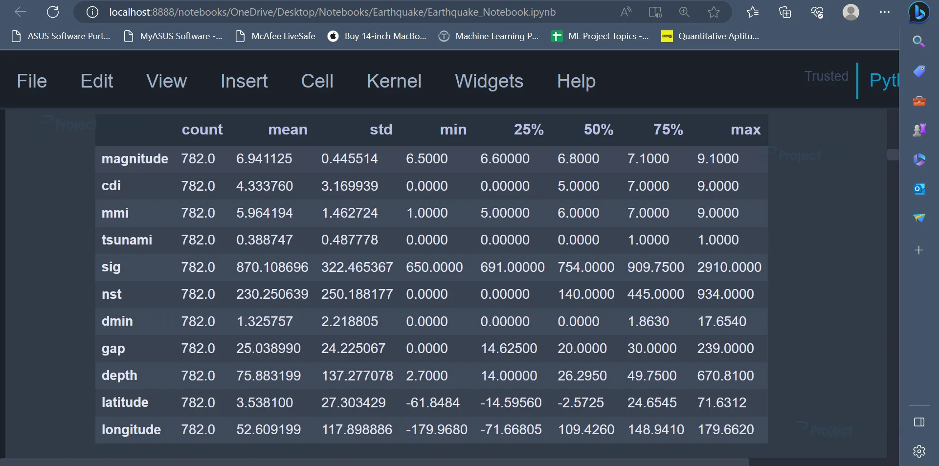
4. Apart from the info() function, the describe() function can also be used to get statistical information about the dataset.

data.describe().transpose()

Output:

The describe() function gives statistical insights like min value, max value, mean value, standard deviation etc., for all the attributes belonging to the dataset.

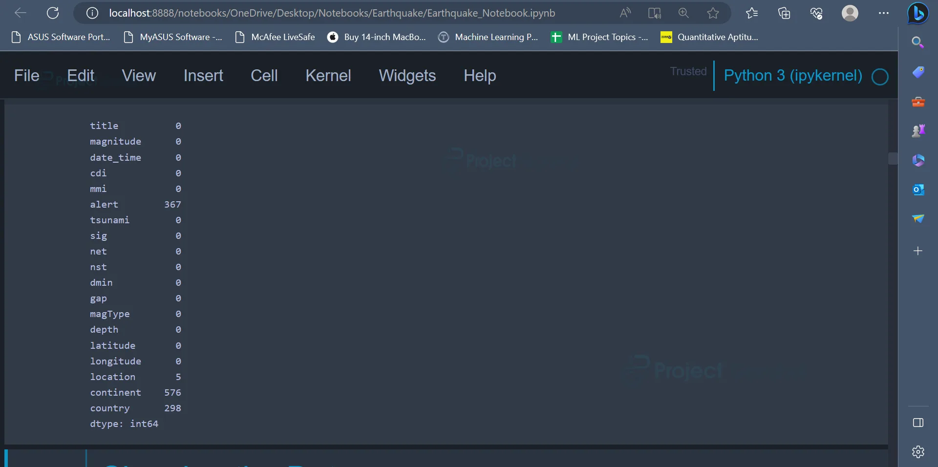
5. The isnull() function can be used to find out if there are any null values present in the dataset and the aggregate function sum() is used to get the total number of null values in each attribute of the dataset.

data.isnull().sum()

Output

The output image displays the total number of null values in all the attributes of the dataset. The columns alert, continent, and country have 367, 576 and 298 null values, respectively.

6. After gaining some basic insights about the data, we can go ahead and clean the dataset. Cleaning the dataset will help in transforming it into a better form which can be later used to train various machine learning models.

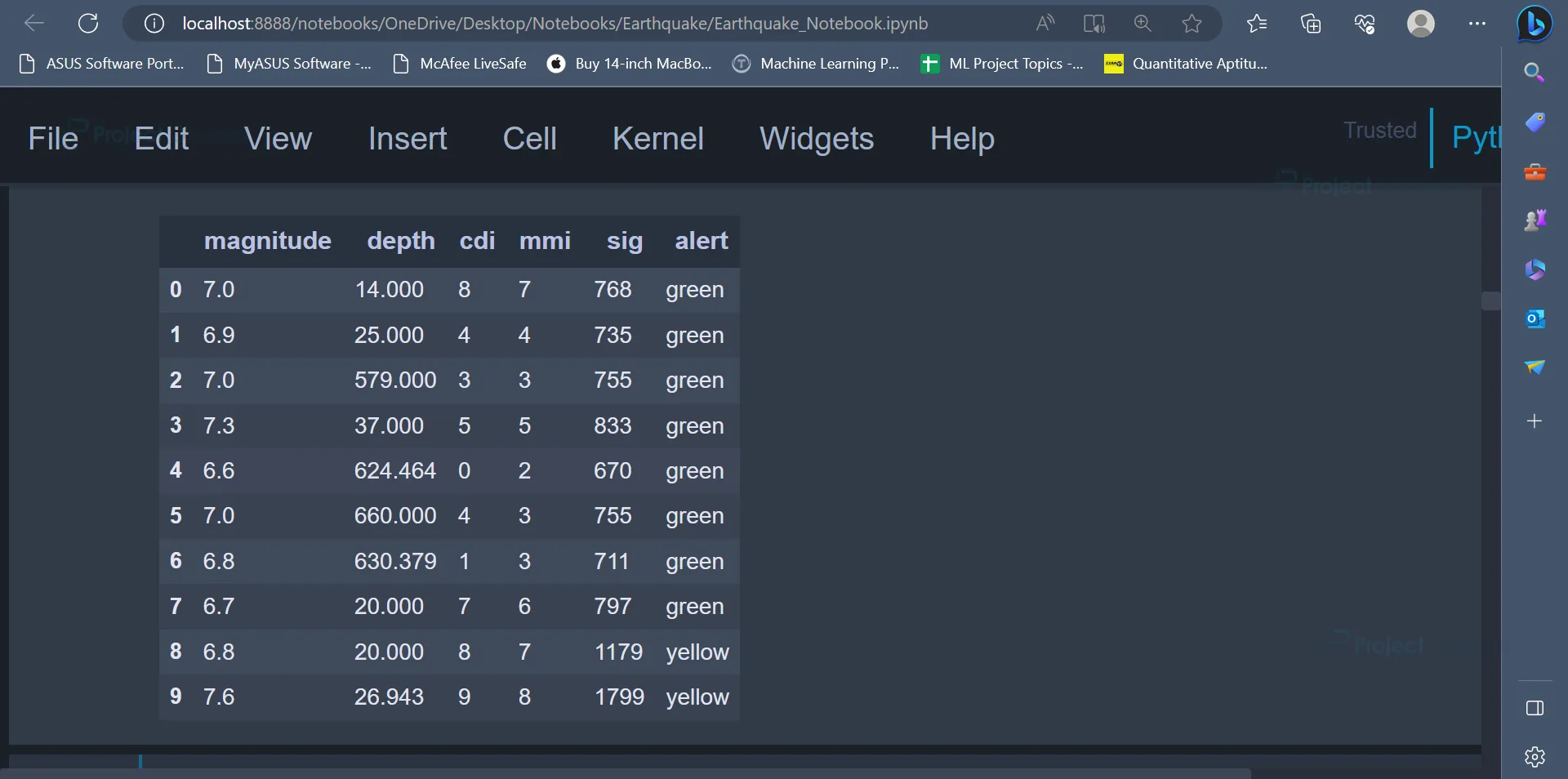
features = ["magnitude", "depth", "cdi", "mmi", "sig"]
target = "alert"
data = data[features + [target]]
data.head()

Output

In the code given above, we create a list called features which contains the attributes named magnitude, depth, cdi, mmi, sig. We will be using machine learning models to predict the values of the alert attribute.

The alert attribute is stored in a variable called target. In the next step, we will create a dataframe and select only those columns/attributes mentioned in the features list along with the target variable.

The first ten rows of the new dataframe can be displayed using the head() function.

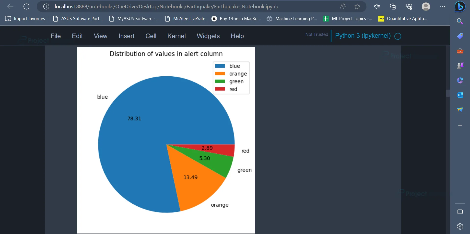
7. The count of all the values present in the alert attribute can be displayed using a pie chart.

plt.figure(figsize = (6,12))
plt.pie(x = data[target].value_counts(), labels = ['blue','orange','green','red'], autopct = '%.2f')
plt.title("Distribution of values in alert column")
plt.legend()
plt.show()

Output:

The pie chart displays the distribution of various values present in the alert column. The percentage of occurrence of various values is blue = 78.31%, orange = 13.49%, green = 5.30%, red = 2.89%.

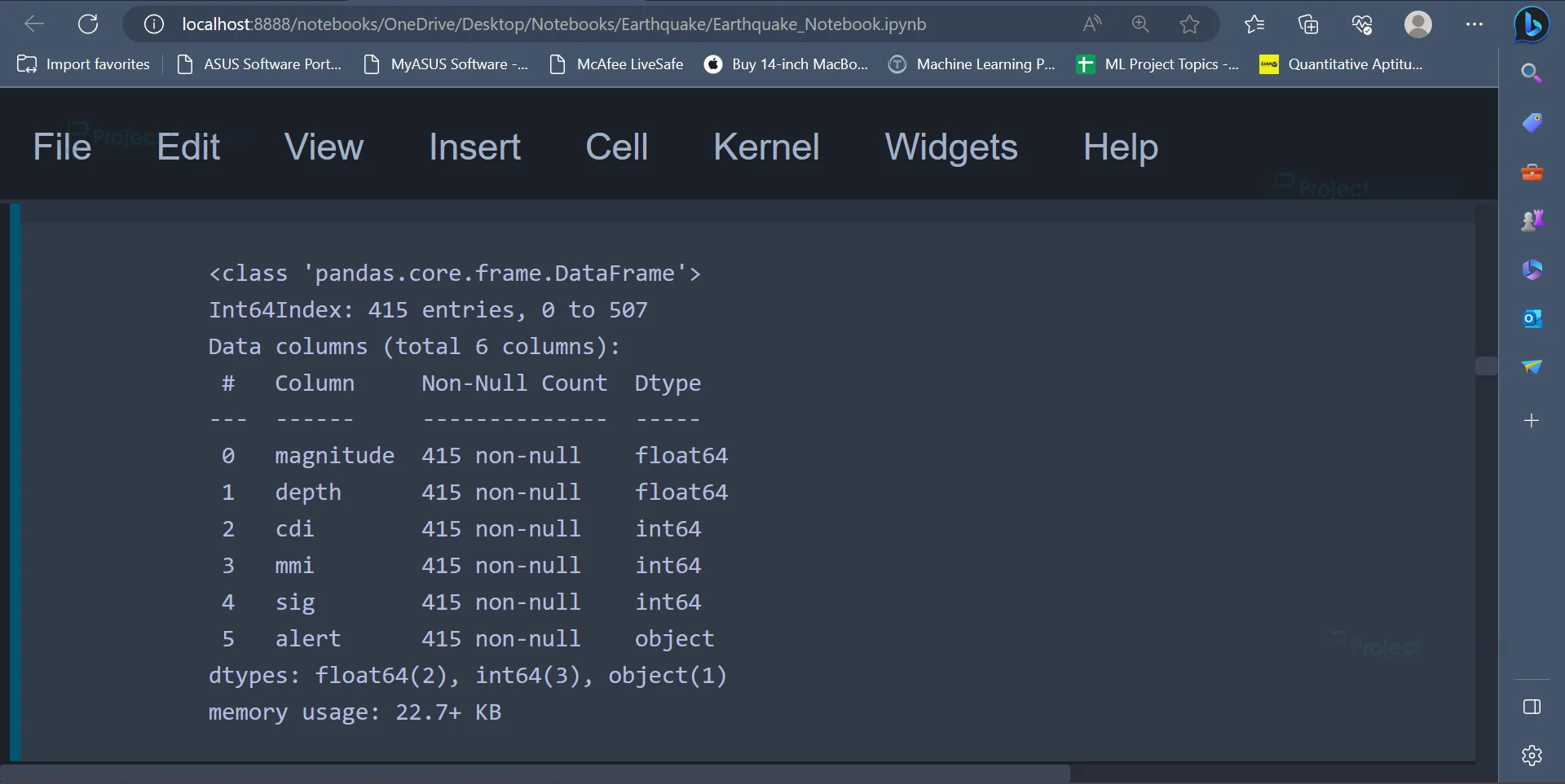
8. Earlier, we had seen that some attributes in the dataset contain certain null values. Since there are not many null values, these values can be removed from the dataset using the dropna() function.

data.dropna(inplace=True)
data.info()

Output:

The null values are removed using the dropna() function, and in the next line, the info() function is used to get some basic information about the dataset.

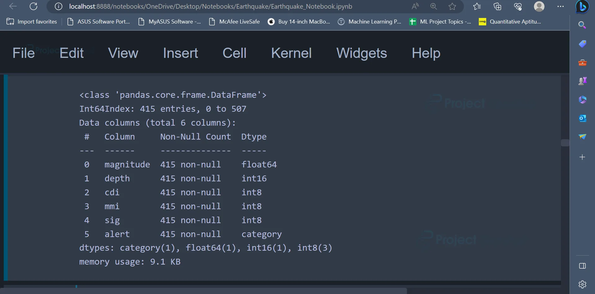
9. In the next step, we will be pre-processing the data. In this step, data types of certain attributes will be changed. In the code, the attributes cdi, mmi, sig are converted from type int64 to type int8, and the attribute depth is converted from type float64 to int16. The attribute alert is also converted from type object to category. These transformations are mostly done for memory optimization. Other reasons to convert the data types would be, to represent the data in a better way using integer numbers rather than floating point numbers.

data = data.astype({'cdi': 'int8', 'mmi': 'int8', 'sig': 'int8', 'depth': 'int16', 'alert': 'category'})
data.info()

Output:

Once the data types of the attributes are converted, the info() function can be used to display the information about the attributes and their data types.

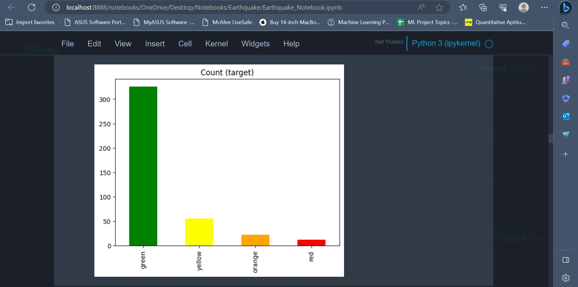
10. Now, let’s check the count of various values present in the target (alert) column. We can use the bar plot for this purpose.

data[target].value_counts().plot(kind='bar', title='Count (target)', color=['green', 'yellow', 'orange', 'red']);

Output:

The output image is a bar plot displaying the count of all the values in the alert attribute. The values are green, yellow, orange, and red. The majority of the values are green, followed by yellow, orange and red.

11. In the previous step, it was seen that the most frequently occurring value in the alert attribute is the value green. This indicates the alert attribute is imbalanced, i.e. values in the alert attribute do not have the same number of occurrences. To overcome the problem of imbalance in the alert attribute, we can perform over-sampling. Over sampling also helps the model to perform well since it eliminates the chances of being biased towards the value which has the highest occurrence.

X = data[features]
y = data[target]

X = X.loc[:,~X.columns.duplicated()]

sm = SMOTE(random_state=42)
X_res, y_res= sm.fit_resample(X, y,)

y_res.value_counts().plot(kind='bar', title='Count (target)', color=['green', 'orange', 'red', 'yellow']);

In the first two lines, the variable X is initialised to a dataframe named data. This feature is a list of attributes which have been specified earlier.

The variable y is initialised with the target (alert) column of the dataframe.

In the next line, the code removes any duplicated columns from the X value. Only those columns which are not duplicated will be stored in X.

Once this is done, we create a new instance of the SMOTE algorithm. SMOTE stands for Synthetic Minority Oversampling Technique. This is a commonly used technique used to solve the problem of class imbalance in Machine Learning.

After creating an instance of the SMOTE algorithm, this instance can be used to apply the SMOTE resampling technique to variables X and y. The value obtained after applying the SMOTE algorithm is stored in variables named x_res and y_res, respectively.

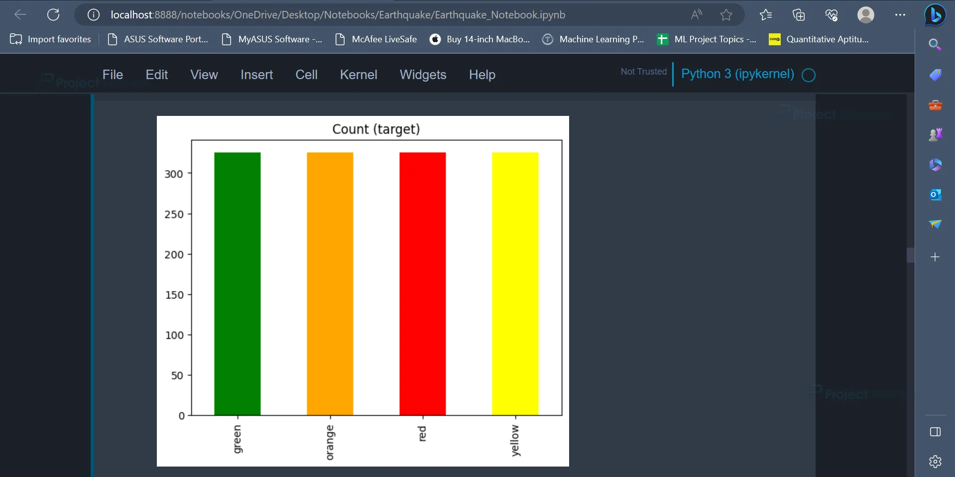
Once this is done, we can use the barplot to plot the values present in the y_res variable.

Output:

From the barplot, it is evident that all the values present in the y_res variable have equal number of occurrences now.

12. Moving forward, we can split the data into training data and testing data using the train_test_split() function.

from sklearn.model_selection import train_test_split
X_train, X_test, y_train, y_test = train_test_split(X_res, y_res, test_size=0.2, random_state=42)

Note that, in the above code, we have used the variables X_res and y_res as independent variables and dependent variables respectively. We use X_res and y_res since it does not have the problem of imbalance in the alert attribute.

The original dataframe faced the problem of imbalance in the alert attribute.

13. Before we start implementing models on our dataset, we will have to bring the data to a standard scale, which would eventually help the machine-learning model understand the data in a better way.

This can be done using the StandardScaler() function.

from sklearn.preprocessing import StandardScaler
scaler = StandardScaler()
X_train = scaler.fit_transform(X_train)
X_test = scaler.transform(X_test)

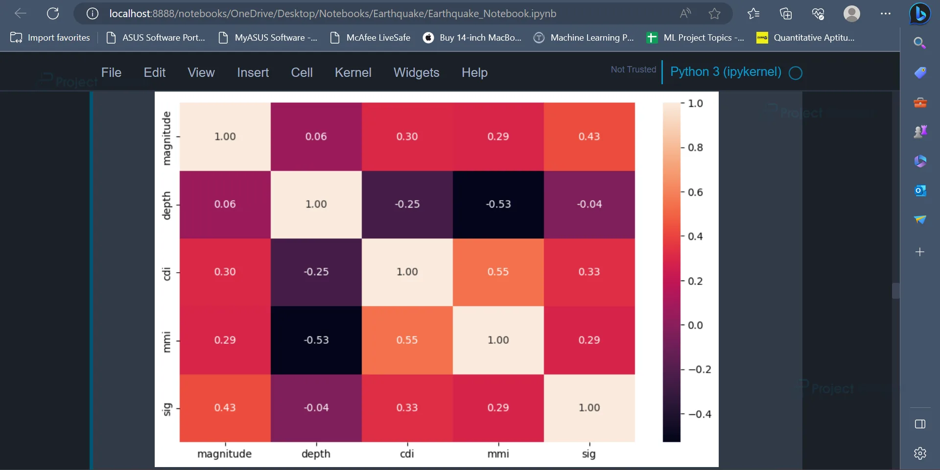
14. We can plot the correlation between various values present in the dataset. The correlation matrix indicates the relationship between various variables present in the dataset and how each variable is affected by every other variable.

It can also be plotted using the below code.

plt.figure(figsize = (10,6))
sns.heatmap(data.corr(), annot=True, fmt=".2f")
plt.plot()

Output:

The correlation matrix represents the correlation coefficients between various values present in the dataset

15. In the next step, we can train various Machine Learning models on the training dataset, and the performance of these models can be evaluated using the testing dataset.

models = []
from sklearn.tree import DecisionTreeClassifier
dt = DecisionTreeClassifier(random_state=42)
dt.fit(X_train, y_train)

Predictions from the model can be made using the predict() method.

The performance of the models can be evaluated using metrics accuracy_score, classification_report, and confusion_matrix.

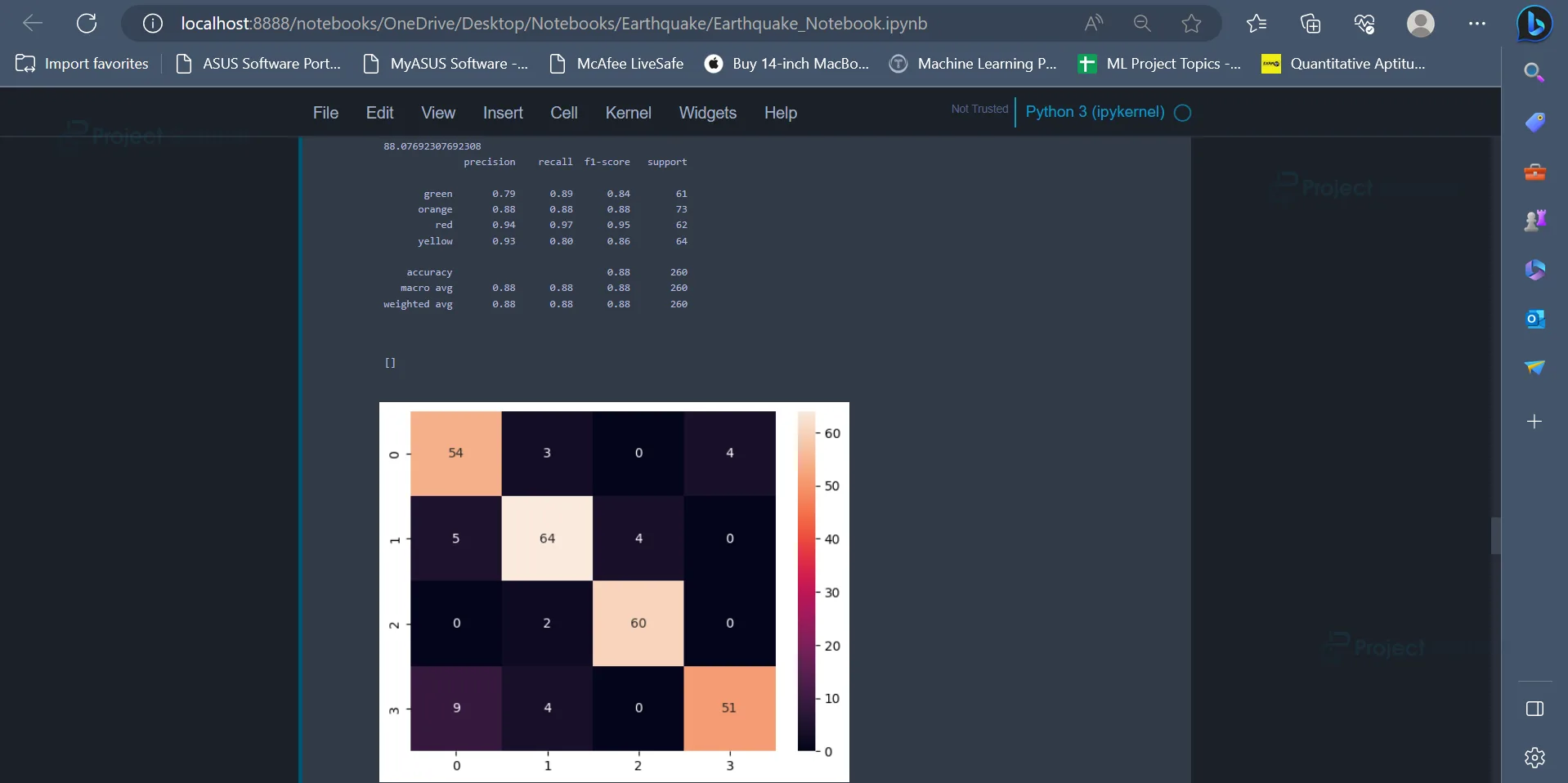
from sklearn.metrics import classification_report, confusion_matrix, accuracy_score
dt_pred = dt.predict(X_test)
print(accuracy_score(dt_pred,y_test)*100)
print(classification_report(dt_pred, y_test))
sns.heatmap(confusion_matrix(dt_pred, y_test), annot = True)
plt.plot()

Output:

The values present in the diagonal of the confusion matrix (54,64,60,51) represent the number of data points which have been correctly classified by the model. From the accuracy score, it is evident that Decision Tree Classifier has an accuracy of 88.07%.

16. The next model which we will be implementing is KNN.

from sklearn.neighbors import KNeighborsClassifier
knn = KNeighborsClassifier()
knn.fit(X_train, y_train)

The predictions from the model are made in a way similar to how it was made earlier.

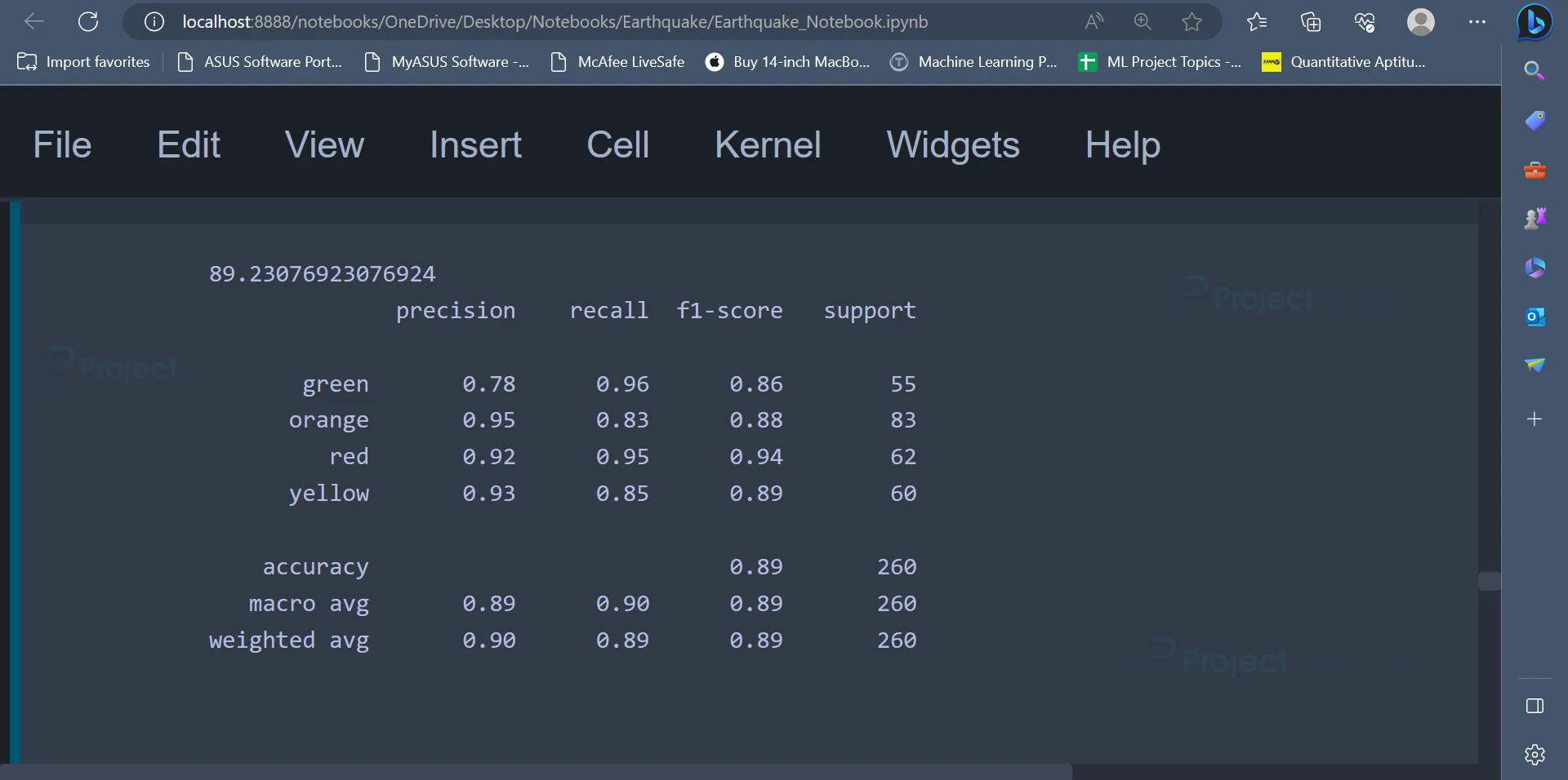
knn_pred = knn.predict(X_test)
print(accuracy_score(knn_pred, y_test)*100)
print(classification_report(knn_pred, y_test))
sns.heatmap(confusion_matrix(knn_pred, y_test), annot = True)
plt.plot()

Output:

The confusion matrix and accuracy score can be displayed like earlier. From the output, it is evident that KNN has an accuracy of 89.23%.

17. After using the KNN algorithm, we can use the Random Forest Classifier on the dataset.

from sklearn.ensemble import RandomForestClassifier
rf = RandomForestClassifier(random_state=42)
rf.fit(X_train, y_train)

The predictions from the Random Forest Classifier can be made using the predict() method. The confusion matrix and accuracy score can be displayed like earlier.

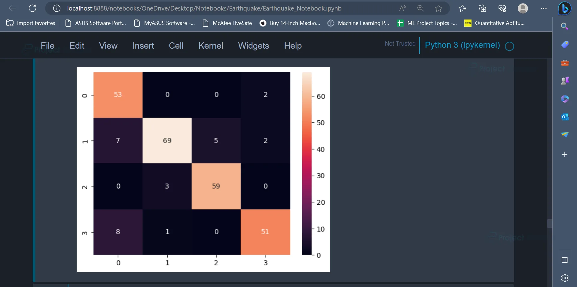
rf_pred = rf.predict(X_test)
print(accuracy_score(rf_pred, y_test)*100)
print(classification_report(rf_pred, y_test))
sns.heatmap(confusion_matrix(rf_pred, y_test), annot = True)
plt.plot()

Output:

It can be seen that the Random Forest Classifier has an accuracy of 91.15%.

18. The last model that we will be implementing is the Gradient Boosting Classifier.

from sklearn.ensemble import GradientBoostingClassifier
gb = GradientBoostingClassifier(random_state=42)
gb.fit(X_train, y_train)

The confusion matrix and accuracy can be displayed like earlier.

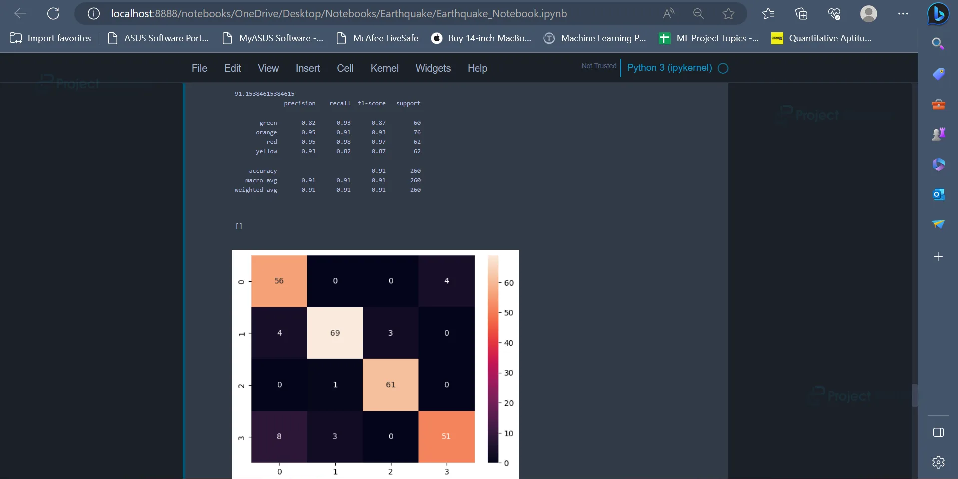
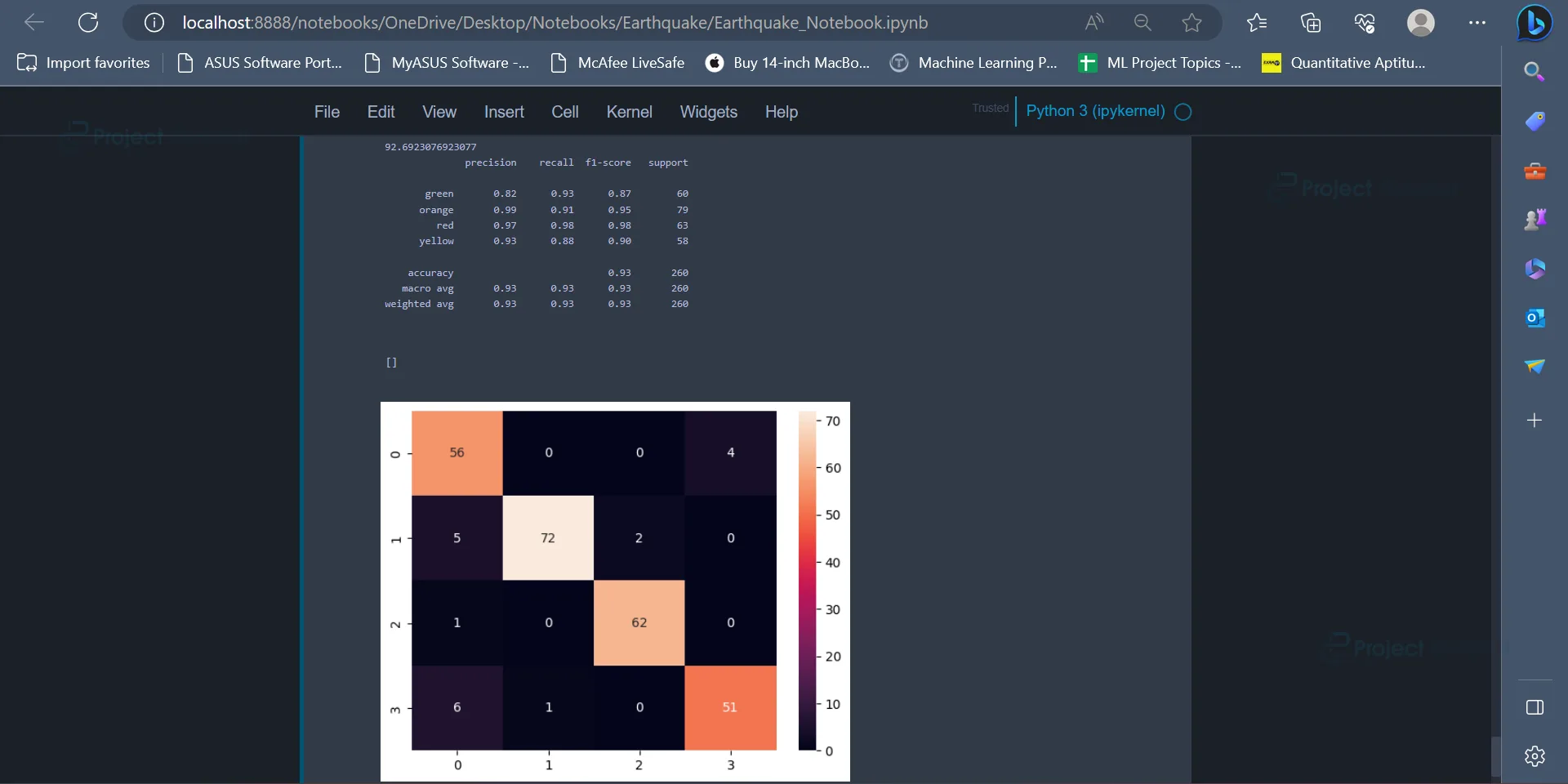
gb_pred = gb.predict(X_test)
print(accuracy_score(gb_pred, y_test)*100)
print(classification_report(gb_pred, y_test))
sns.heatmap(confusion_matrix(gb_pred, y_test), annot = True)
plt.plot()

Output:

The Gradient Boosting Algorithm has an accuracy of 92.69%.

Conclusion

In conclusion, machine learning techniques have shown promising results in the prediction of earthquakes. By analysing various data sources like seismic recordings, geospatial information etc., machine learning models can learn patterns, trends, and relationships, which can help in identifying potential earthquake occurrences.

While machine learning models can assist in the prediction of earthquakes, it is important to note that it is an ongoing research area and achieving reliable as well as accurate predictions remains a complex task. Collaborative efforts between domain experts and machine learning engineers are crucial to advance the field and develop robust models which can help in the early detection of earthquakes.