Heart Disease Prediction using Machine Learning

With this Machine Learning Project, we will be doing heart disease prediction. For this project, we are using Logistic Regression, Decision Tree Classifier, and Random Forest Classifier.

So, let’s build this system.

Heart Disease Prediction

Machine learning is defined as the process of “manipulating and retrieving implicit, previously unknown/known, and possibly important information about data.” The field of machine learning is quite vast and complicated, and its applications and scope are constantly growing. Machine learning makes use of a number of classifiers from supervised, unsupervised, and ensemble learning to forecast and assess the precision of the given dataset. Many people will find the information useful, so we can use it in our HDPS project.

These days, a wide variety of disorders that potentially harm your heart are referred to as cardiovascular diseases. According to the World Health Organization, there are 17.9 million CVD-related deaths worldwide.

Adult deaths are primarily brought on by it. With the aid of their medical history, our initiative can identify individuals who are most likely to be diagnosed with heart disease. It can assist in identifying diseases with fewer medical tests and efficient treatments so that patients can be treated appropriately. It can identify anyone who is experiencing any heart disease symptoms, such as chest pain or high blood pressure.

Three data mining techniques—logistic regression, decision trees that are superior to earlier models, and random forest classifier—are the major emphasis of this study. Our project’s accuracy for a system using a single data mining technique is about to 86%. Thus, the accuracy and efficiency of HDPS were improved by applying more data mining techniques.

Based on the patient’s medical characteristics, such as gender, age, chest discomfort, fasting blood sugar level, etc., this study seeks to determine if the patient is likely to be diagnosed with any cardiovascular heart condition. The attributes and medical history of the patient are contained in a dataset chosen from the UCI repository. We make a prediction about the patient’s potential heart condition using this dataset. In order to forecast this, we utilize a patient’s medical characteristics to categorize him or determine whether he is likely to get one of 14 heart disorders. Three algorithms—Logistic Regression, Decision Tree, and Random Forest Classifier—are used in this project because these algorithms seem to perform the best. The method with the highest accuracy, Logistic, has a precision rate of 86.88%.

Let’s take a look at our best algorithm which is Logistic Regression.

Logistic Regression

Logistic regression is based on the basic mathematical concept of the logit or the natural logarithm of an odds ratio. The simplest example of logit is based on a 2×2 contingency table.

Logistic regression, in particular, is a useful method for formulating and evaluating hypotheses about correlations between one or more categorical or continuous predictor variables and a categorical result variable. The plot of such data shows two parallel lines, each of which corresponds to a dichotomous outcome value for continuous predictor X and dichotomous outcome variable Y in the simplest case. It is difficult to describe the two parallel lines using an ordinary least squares regression equation because of the dichotomy of results. As an alternative, one might categorize the predictor and figure out what each category’s mean of the outcome variable is. The resulting scatter plot of category means will be linear in the middle and curved at the extremities, as one might anticipate from a conventional scatter plot.

Project Prerequisites

The requirement for this project is Python 3.6 installed on your computer. I have used a Jupyter notebook for this project. You can use whatever you want.
The required modules for this project are –

1. Numpy(1.22.4) – pip install numpy
2. Pandas(1.5.0) – pip install pandas
3. Seaborn(0.9.0) – pip install seaborn
4. SkLearn(1.1.1) – pip install sklearn

That’s all we need for our project.

Heart Disease Prediction Project & DataSet

Please download source code and dataset that will be required in heart disease prediction project. We will require a csv file for this project. You can download the dataset and the jupyter notebook from the following below: Heart Disease Prediction Project

Steps to Implement

1. Import the modules and the libraries. For this project, we are importing the libraries numpy, pandas, and sklearn and metrics. Here we also read our dataset and we are saving it into a variable.

import numpy as np #importing the numpy module which will be used in this project
import pandas as pd#importing the pandas module which will be used in this project
import matplotlib.pyplot as plt#importing the matplotlib module which will be used in this project
import seaborn as sns#importing the seaborn module which will be used in this project
from sklearn.model_selection import train_test_split#importing the sklearn module which will be used in this project
 

2. Here we are reading our dataset. And we are printing our dataset

dataframe = pd.read_csv('dataset.csv')#reading our dataset using read_csv function
dataframe.head() #printing the first 5 columns of our dataset using head function

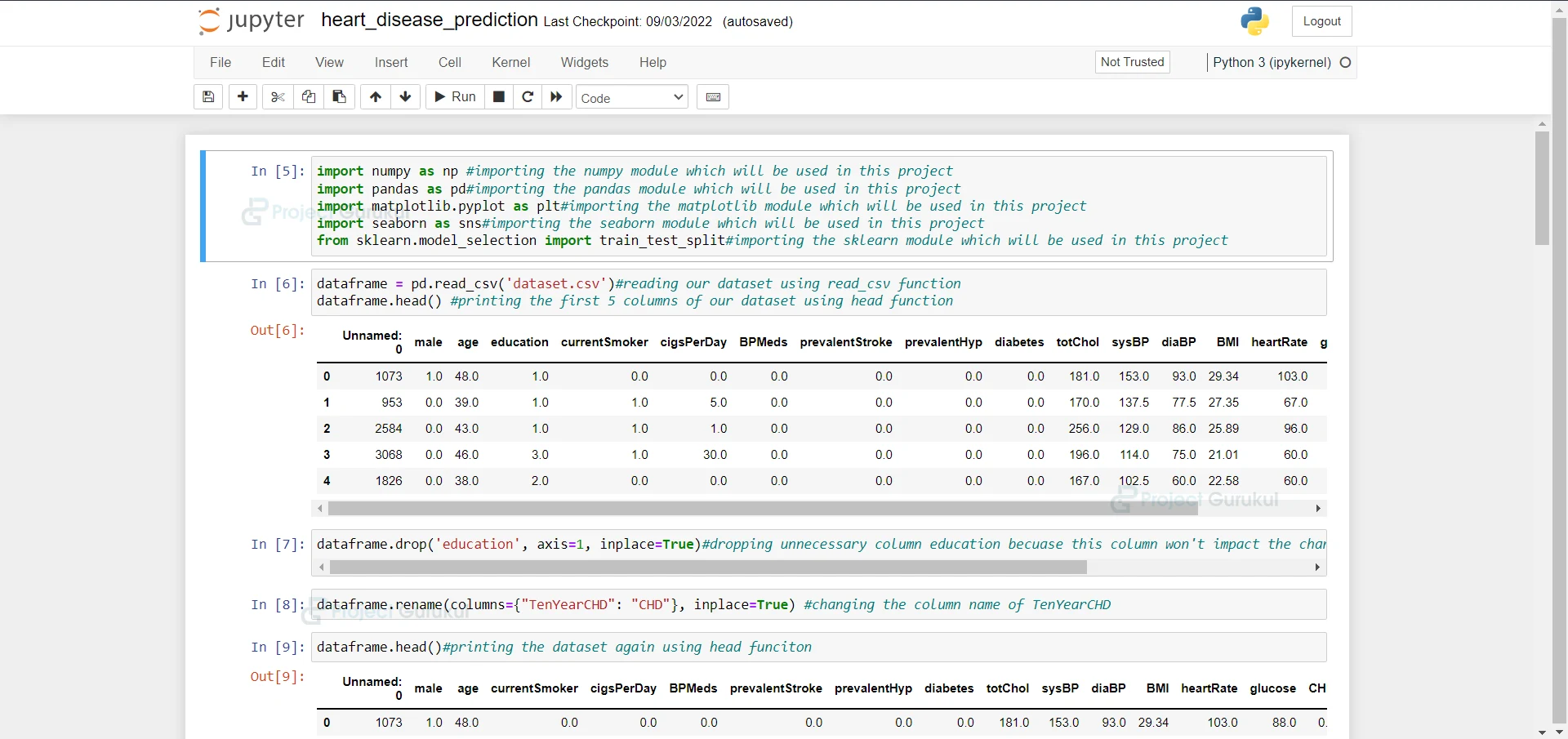
3. Here we are dropping unnecessary column education because this column won’t impact the chances of a person having a heart attack.

dataframe.drop('education', axis=1, inplace=True)#dropping unnecessary column education becuase this column won't impact the chances of a person having a heart attack
 

4. Here we are renaming a column to CHD.

 
dataframe.rename(columns={"TenYearCHD": "CHD"}, inplace=True) #changing the column name of TenYearCHD

5. Here we are printing the dataset again.

dataframe.head()#printing the dataset again using head funciton

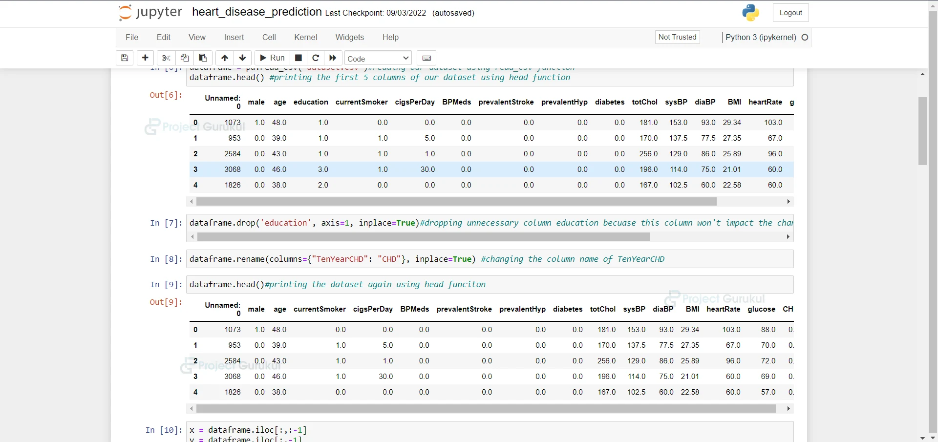
6. Here we are dividing the dataset into testing and training datasets.

x = dataframe.iloc[:,:-1]
y = dataframe.iloc[:,-1]
X_train, X_test, y_train, y_test = train_test_split(x, y, test_size=0.20)
 
train_data = pd.concat([X_train, y_train], axis=1)
test_data = pd.concat([X_test, y_test], axis=1)
 

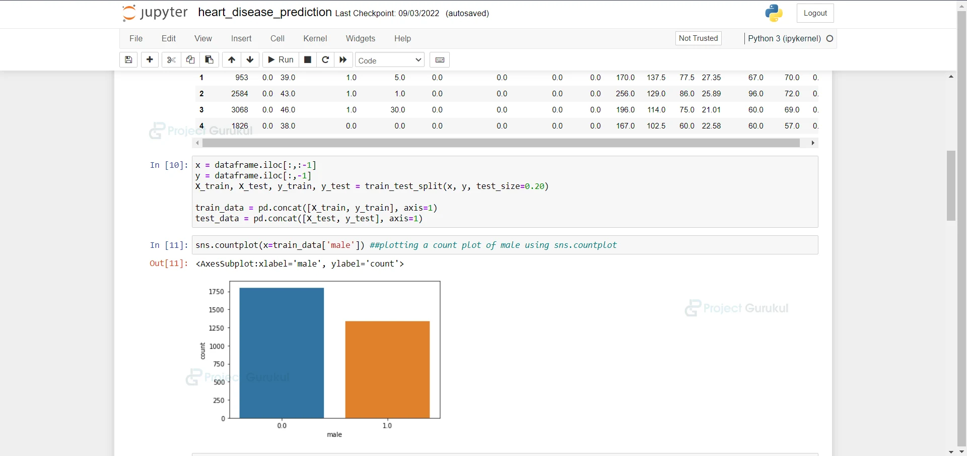
7. Here we are plotting a count plot of males using sns.countplot.

sns.countplot(x=train_data['male']) ##plotting a count plot of male using sns.countplot

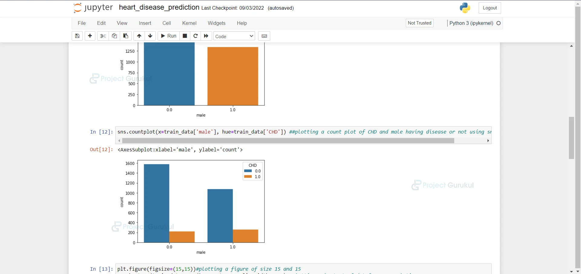
8. Here we are plotting a count plot of CHD and males having a disease or not using sns.countplot.

sns.countplot(x=train_data['male'], hue=train_data['CHD']) ##plotting a count plot of CHD and male having disease or not using sns.countplot
 

9. Here we are plotting a heatmap of data frame correlation

plt.figure(figsize=(15,15))#plotting a figure of size 15 and 15
 
sns.heatmap(train_data.corr(), annot=True, linewidths=0.1) #plotting a heatmat of dataframe correlation

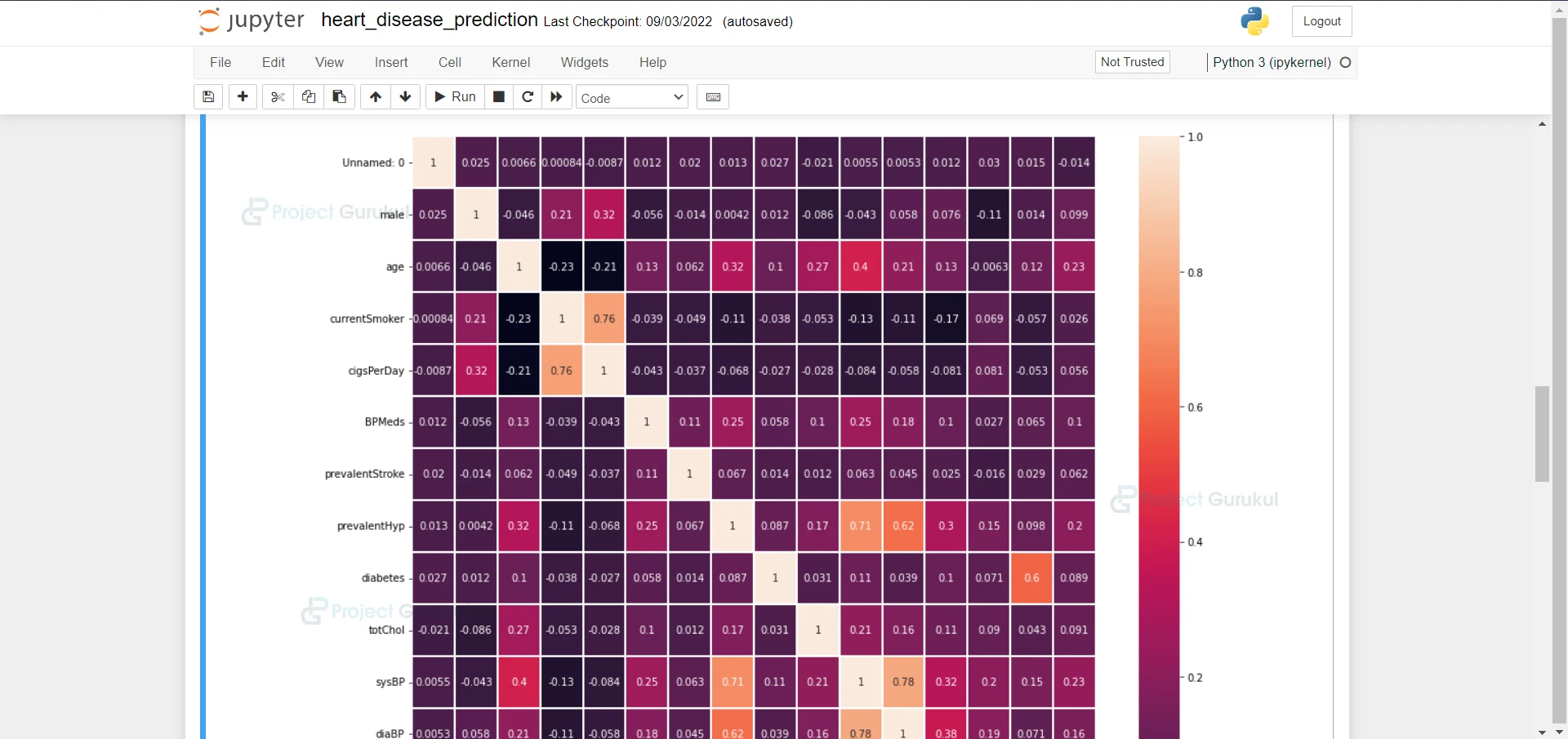
10. Here we are dropping the column because they are correlated very highly.

train_data.drop(['currentSmoker', 'diaBP'], axis=1, inplace=True)#dropping the column becuase they are correlated very high
 

11. Here we are deleting the outliers values in different columns of training data.

train_data = train_data[~(train_data['sysBP'] > 220)] #deleting the outliers values in sysBP of training data
train_data = train_data[~(train_data['BMI'] > 43)]#deleting the outliers values in BMI of training data
train_data = train_data[~(train_data['heartRate'] > 125)]#deleting the outliers values in heartRate of training data
train_data = train_data[~(train_data['glucose'] > 200)]#deleting the outliers values in glucose of training data
train_data = train_data[~(train_data['totChol'] > 450)]#deleting the outliers values in totChol of training data
 

12. Here we are taking all the columns which are to be standardized in an array

from sklearn.preprocessing import StandardScaler #importing the standard scaler library
scaler = StandardScaler()
train_data[cols_to_standardise] = scaler.fit_transform(train_data[['age','totChol','sysBP','BMI', 'heartRate', 'glucose', 'cigsPerDay']])#taking all the columns which are to be standardise in an array
 

13. Here we are fitting the data and filling any null values in the test dataset.

test_data.drop(['currentSmoker', 'diaBP'], axis=1, inplace=True)
 
imputer = SimpleImputer(strategy='most_frequent')#Creating an instance of simple Imputer which will be used to fill the null vlaues
test_data = pd.DataFrame(imputer.fit_transform(test_data))#fitting the data and filling any null values in the test dataset
 

14. Here we are taking all columns which are to be standardized in an array.

test_data[cols_to_standardise] = scaler.fit_transform(test_data[['age','totChol','sysBP','BMI', 'heartRate', 'glucose', 'cigsPerDay']])#taking all the columns which are to be standardise in an array

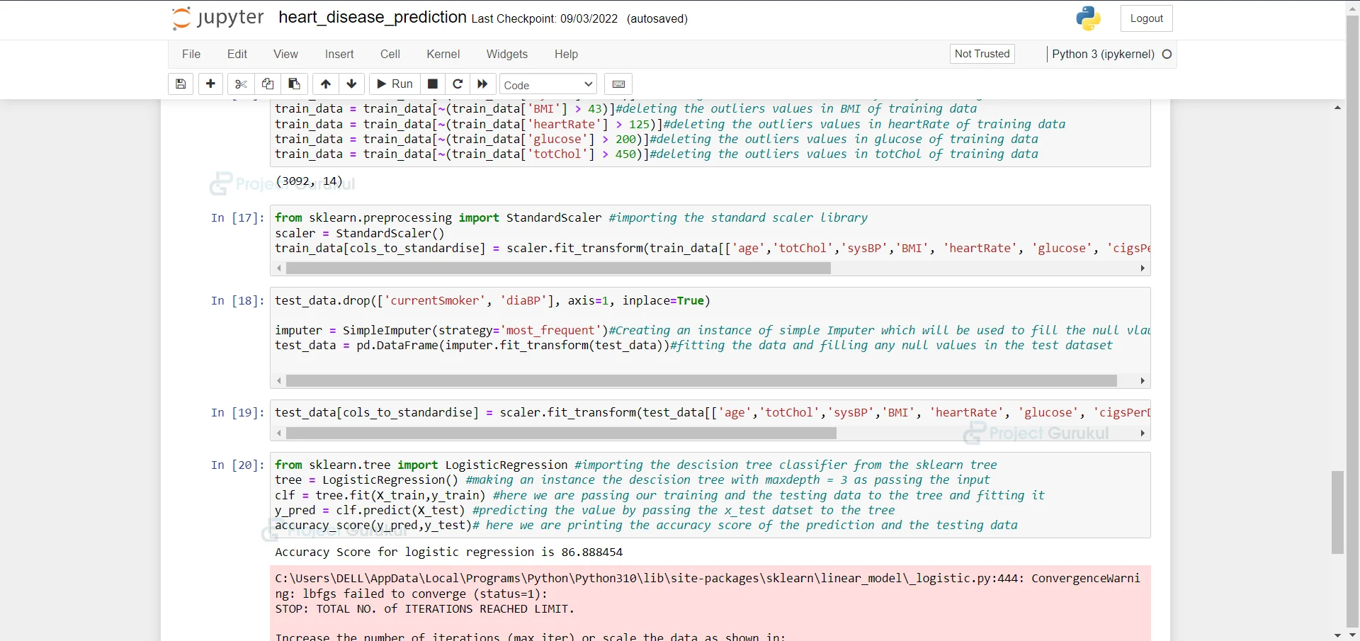
15. Importing the Logistic Regression from sklearn and fitting our training and testing data into it and we are printing the accuracy of the model.

 
from sklearn.tree import LogisticRegression #importing the descision tree classifier from the sklearn tree 
tree = LogisticRegression() #making an instance the descision tree with maxdepth = 3 as passing the input
clf = tree.fit(X_train,y_train) #here we are passing our training and the testing data to the tree and fitting it
y_pred = clf.predict(X_test) #predicting the value by passing the x_test datset to the tree 
accuracy_score(y_pred,y_test)# here we are printing the accuracy score of the prediction and the testing data
 

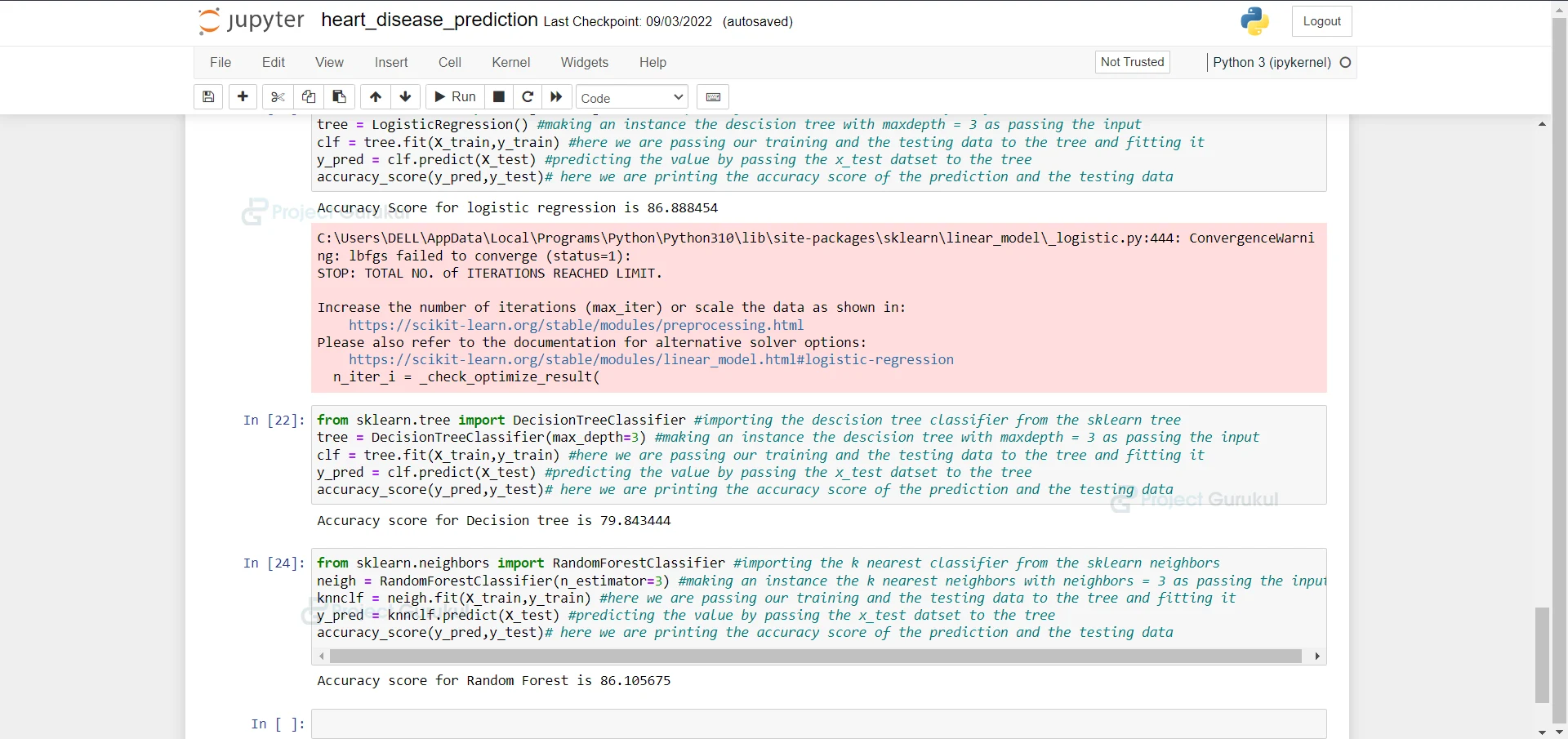
16. Importing the Decision Tree Classifier from sklearn and fitting our training and testing data into it and we are printing the accuracy of the model.

from sklearn.tree import DecisionTreeClassifier #importing the descision tree classifier from the sklearn tree 
tree = DecisionTreeClassifier(max_depth=3) #making an instance the descision tree with maxdepth = 3 as passing the input
clf = tree.fit(X_train,y_train) #here we are passing our training and the testing data to the tree and fitting it
y_pred = clf.predict(X_test) #predicting the value by passing the x_test datset to the tree 
accuracy_score(y_pred,y_test)# here we are printing the accuracy score of the prediction and the testing data

17. Importing the Random Forest Classifier from sklearn and fitting our training and testing data into it and we are printing the accuracy of the model.

 
from sklearn.neighbors import RandomForestClassifier #importing the k nearest classifier from the sklearn neighbors 
neigh = RandomForestClassifier(n_estimator=3) #making an instance the k nearest neighbors with neighbors = 3 as passing the input
knnclf = neigh.fit(X_train,y_train) #here we are passing our training and the testing data to the tree and fitting it
y_pred = knnclf.predict(X_test) #predicting the value by passing the x_test datset to the tree 
accuracy_score(y_pred,y_test)# here we are printing the accuracy score of the prediction and the testing data

Summary

In this Machine Learning project, we develop a heart disease prediction model. For this project, we are using Logistic Regression, Decision Tree Classifier, and Random Forest Classifier. We hope you have learned something new from this project.