Food Classification using Deep Learning

With this Deep Learning Project, we will be developing a food classification system. For this project, we are using Convolutional Neural Networks.

So, let’s build this system.

Food Image Classification

We “consume with our eyes,” as is often remarked. Our digital experience is becoming more and more photo-driven due to the ongoing growth of social media platforms like Instagram (which has 500 million daily active users as of this writing). Of these, over 360 million of these photos are pictures of food (looking at just food). More than 88% of poll respondents who responded in 2015 believed that food was the defining factor in deciding on travel locations and said that food images almost entirely drive dining experiences, food festivals, culinary lessons, and the emergence of gastro-tourism.

The food search experience is mainly chaotic and challenging to browse due to the fact that the majority of these photographs are unidentified and may or may not be connected to a place or a tag. In order to improve image labeling, this project is about the categorization of food images using convolutional neural networks (CNNs). The project’s objective is to produce the appropriate label classification of a food image given an image of a plate as the model’s input.

Image Dataset

The Food-101 dataset, which contains 1000 photos for each kind of food, was utilized to create a total of 101,000 images. A total of 75,750 training photos and 25,250 test images made up the 1000 images for each class. Of these, 250 were manually inspected test images and 750 were purposefully noisy training images.

The Food-101 dataset poses a few more difficulties than the 10-class ImageNet food image dataset. For one, the ImageNet food image dataset contains relatively distinct and few food categories (apple, banana, broccoli, burger, egg, french fries, hot dog, pizza, rice, and strawberry), while Food-101 contains some food items that are similar in both content and presentation (e.g. pho vs. ramen). In order to encourage models to be resilient to labeling anomalies, the training dataset images also comprised mislabeled photos and had very different lighting, color, and size characteristics. Instead of using the ImageNet dataset directly, we additionally used ImageNet weights to increase model accuracy. Images were correctly normalized and resized, either to 128×128 or 256×256 in the first model implementations when employing transfer learning for model specification. To prevent overfitting, image data was enhanced using rotation, shifting, and horizontal flipping. The custom model preprocessing routines, which were implementations of the image preprocessing in the original model publications, were also used to preprocess images during transfer learning.

CNN (Convolutional Neural Networks)

We chose CNN for this project since it appears to perform better than every other algorithm when it comes to object detection in photos than any other approach. Compared to other algorithms, it requires incredibly little processing. Consider brain neurons when attempting to comprehend CNN. The CNN model was developed and taught in a similar manner to how our brains develop over time. We feed the brain information, and the brain uses neurons to train itself to look for key elements of the information. The CNN algorithm trains its neurons in a similar manner.

A machine learning algorithm known as a convolutional neural network may predict the item in an image based on how it has been trained.

Let’s discuss how CNN operates –

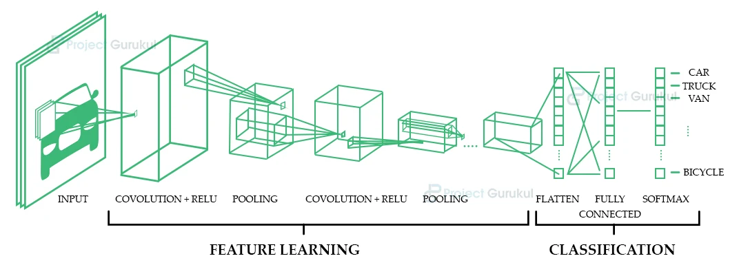
1. Four layers are used to generate CNN. the input layer, which is the first layer. The Convolution layer is the next layer. The pooling layer is the third one.
2. Input Layer: This layer’s input is a simple 2D image. This image is perceived as a matrix of pixels by the computer. as a computer only recognizes an image as a collection of pixels.
3. Convolutional Layer: A convolutional layer is created by a group of filters.

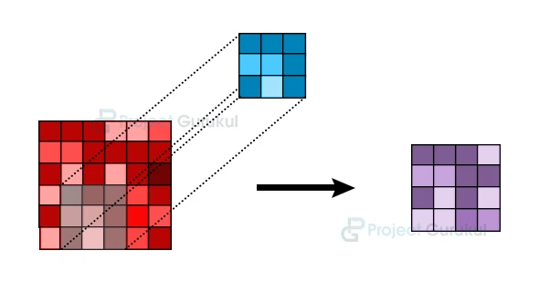
As shown in the picture up top. The M1 matrix is 6×6. There is a 3×3 matrix M2 which is called the filter. We will slide the M2 matrix over the M1 matrix until every pixel is scanned at least once. As we slide the M2 over M1, we will have a 3X3 scanned matrix M3 which is just a patch of M1. Now from this M3 matrix, our convolutional layer will find important features from the M3 matrix in numeric form. It is calculated by multiplying the weight of the filter with the M3 matrix. The result is stored in matrix M4 as seen in the picture.

This is how the Convolutional layer works.

4. Pooling layer: The data matrix is downsampled using the pooling layer. It is applied to lower the matrix’s parameter count. It is done to prevent overfitting, conserve memory, and streamline computation.
Convolution and pooling are both carried out in the same manner. The only distinction is that in this case, we will either take the patch’s greatest value or its average value. There are two types of pooling based on this:
MAX POOLING – Here, we take the patch matrix’s maximum value.

AVERAGE POOLING – Here, we take the patch matrix’s average value.

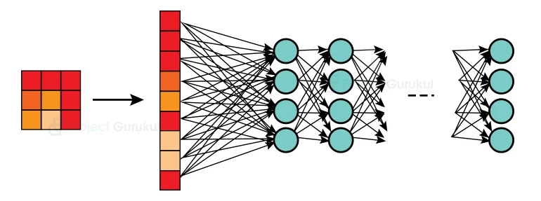
5. Fully Connected layer: This layer obtains the class score by flattening the matrix that was produced in the pooling layer. This flattened matrix, which is a m x 1 matrix, is sent into the neural network’s hidden layers, where the outcome is then predicted.

Model Architecture

The neural network that underlies our model. Convolutional simply means that we are preparing our input before submitting it to the neural network. Convolutional is only an additional layer for neural networks. But this appears to perform better than our old conventional neural networks. We are going to use the Keras library because it contains highly optimized prebuilt CNN so we don’t waste our time writing code for CNN.

We will feed this CNN our training dataset. Our photos will initially be converted into a pixel matrix through this process. because only pixels are recognised by computers. The essential characteristics are then recovered from this matrix once it has been passed to the convolutional layer and the pooling layer. After flattening the resulting matrix, it is then sent to our neural network. There are undiscovered layers in this neural network. The weights in these hidden layers serve as the basis for several computations done by our activation function. If our prediction comes false then it calculates the error, goes back and updates the weights of the filters in the hidden layers. This procedure is repeated until our error becomes so small that it can be ignored.

After that, we pass our test dataset and examine mistakes to see if our model is correctly predicting outcomes.

Finally, to test our model, we send a random image to our neural network and check to see if it properly predicts the image.

Project Prerequisites

The requirement for this project is Python 3.6 installed on your computer. I have used a Jupyter notebook for this project. You can use whatever you want.

The required modules for this project are –

1. Numpy(1.22.4) – pip install numpy
2. Pandas(1.5.0) – pip install pandas
3. Seaborn(0.9.0) – pip install seaborn
4. SkLearn(1.1.1) – pip install sklearn

That’s all we need for our project.

Food Classification Project Code & DataSet

We have provided the dataset for this project that will be required in this food classification project. We will require a csv file for this project. You can download the dataset and the jupyter notebook from the link below.

Please download the food classification dataset and the jupyter notebook from the following link: Food Classification Project

Steps to Implement

1. Import the modules and the libraries. For this project, we are importing the libraries numpy, TensorFlow, and Keras.4

import numpy as np
import tensorflow as tf
from keras.preprocessing.image import ImageDataGenerator

2. Here we are creating an instance of Image Data Generator and then we read our training dataset.

 
## Data preprocessing
## Training Image Preprocessing
 
train_datagen = ImageDataGenerator(featurewise_center=False,
                 samplewise_center=False,
                 featurewise_std_normalization=False,
                 samplewise_std_normalization=False,
                 zca_whitening=False,
                 rotation_range=5,
                 width_shift_range=0.05,
                 height_shift_range=0.05,
                 shear_range=0.2,
                 zoom_range=0.2,
                 channel_shift_range=0.,
                 fill_mode='nearest',
                 cval=0.,
                 horizontal_flip=True,
                 vertical_flip=False,
                 rescale=1/255)
training_set = train_datagen.flow_from_directory(
    'images/train',target_size=(64,64),batch_size=64,class_mode='categorical')

3. Here we are reading our testing dataset.

test_datagen = ImageDataGenerator(rescale=1./255)
test_set = test_datagen.flow_from_directory(
        'images/test',
        target_size=(64, 64),
        batch_size=32,
        class_mode='categorical')

4. Here we are creating our CNN model and we are passing our activation function as relu and softmax.

cnn = tf.keras.models.Sequential()
cnn.add(tf.keras.layers.Conv2D(filters=64 , kernel_size=3 , activation='relu' , input_shape=[64,64,3]))
cnn.add(tf.keras.laye
        rs.MaxPool2D(pool_size=2,strides=2))
cnn.add(tf.keras.layers.Conv2D(filters=64 , kernel_size=3 , activation='relu' ))
cnn.add(tf.keras.layers.MaxPool2D(pool_size=2 , strides=2))
cnn.add(tf.keras.layers.Dropout(0.5))
cnn.add(tf.keras.layers.Flatten())
cnn.add(tf.keras.layers.Dense(units=128, activation='relu'))
cnn.add(tf.keras.layers.Dense(units=9 , activation='softmax'))
cnn.compile(optimizer = 'rmsprop' , loss = 'categorical_crossentropy' , metrics = ['accuracy'])

5. Here we are fitting our model by passing our dataset.

cnn.fit(x = training_set , validation_data = test_set , epochs = 1000)

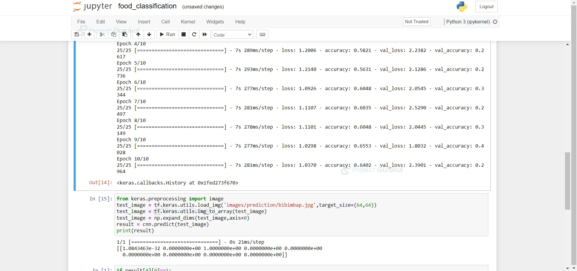
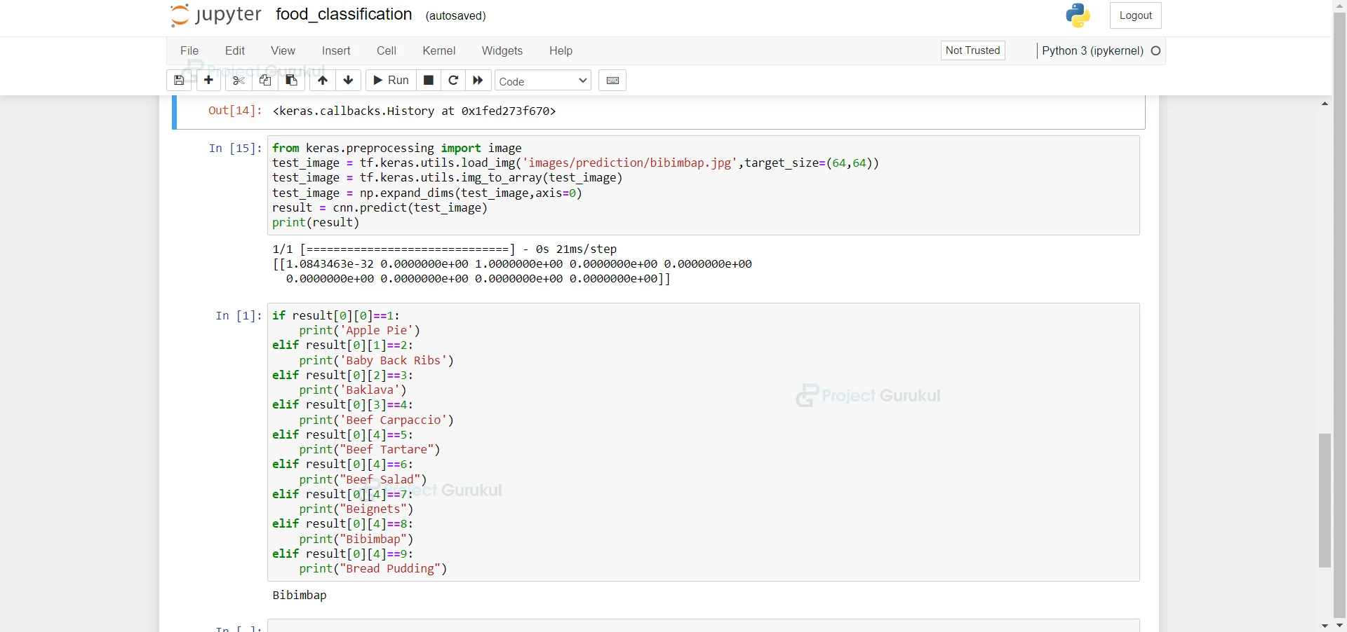
6. Here we are loading our image and then converting our image to array and we are printing our result.

 
from keras.preprocessing import image
test_image = tf.keras.utils.load_img('images/prediction/bibimbap.jpg',target_size=(64,64))
test_image = tf.keras.utils.img_to_array(test_image)
test_image = np.expand_dims(test_image,axis=0)
result = cnn.predict(test_image)
print(result)
 

7. Here we are predicting our food.

 
if result[0][0]==1:
    print('Apple Pie')
elif result[0][1]==2:
    print('Baby Back Ribs')
elif result[0][2]==3:
    print('Baklava')
elif result[0][3]==4:
    print('Beef Carpaccio')
elif result[0][4]==5:
    print("Beef Tartare")
elif result[0][4]==6:
    print("Beef Salad")
elif result[0][4]==7:
    print("Beignets")
elif result[0][4]==8:
    print("Bibimbap")
elif result[0][4]==9:
    print("Bread Pudding")

Summary

In this Machine Learning project, we develop a food classification system using Convolutional Neural Networks. We hope you have learned something new from this project.