Breast Cancer Classification using Machine Learning
FREE Online Courses: Your Passport to Excellence - Start Now
The biggest gift from Artificial Intelligence is in the Healthcare
Develop Breast Cancer Classification system using machine learning that predicts the condition by viewing a digital scan of the patient.
Computer vision and machine learning techniques have shown a high level of accuracy in healthcare applications, but these systems should not be used as only methods of medical examination. These are meant to help doctors, not replace them.
Details about Breast Cancer
When the cells multiply and multiply in an uncontrolled way due to mutation caused in genes that regulate the growth of those cells, the condition termed as cancer. Cancer develops in breast cells known as breast cancer.
Breast cancer accounted for almost 25% of all cancer in recent years.
There are a few kinds of breast cancer that depends on which cells of the breast turn to cancer. The breast is mostly made up of three kinds of cells: lobules, ducts, and connective tissues. Lobules are the gland that produce milk, the tubes carrying the milk to the nipples are ducts. The connective tissue made up of mostly fatty and fibrous tissues, surrounds and holds everything together.
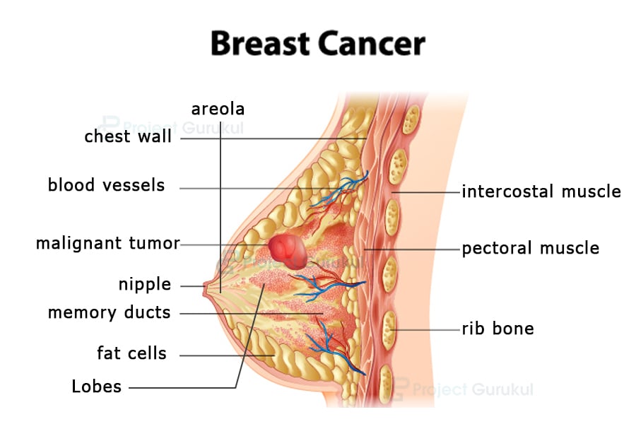
In most cases, the tumor forms in the lobules or duct cells, but can very seldom occur in the connective tissues. This uncontrolled cancer can sometimes travel and infect other healthy breast tissues as well as the lymph nodes under the arms.
There are a few types of breast cancer, most common of them being:
- Invasive ductal carcinoma or IDC which starts in the milk ducts of the breast is the most common type of breast cancer. Cancer can then spread to other regions of the breast.
- Invasive lobular carcinoma or ILC begins in the lobules of the breast. These cells then invade nearby tissues.
Breast Cancer Classification
The key to identify cancer is to identify tumors as malignant and benign, malignant being cancerous and benign being non-cancerous.
Early diagnosis of breast cancer can be very helpful and maybe even life-saving. We are going to build a system which can identify if the tumor is benign or malignant based on the features obtained from several cell images which are mostly based on the cell shape and its geometry. A digitized image of fine needle aspirate (FNA) of breast mass, a type of biopsy procedure used to obtain the features. They describe the characteristics of the cell nuclei present in the image.
Breast Cancer Classification – Machine Learning Dataset
The dataset used is the Breast Cancer Wisconsin (Diagnostic) data set.
Please download dataset for machine learning training and testing in breast cancer classification: Breast Cancer Dataset
Breast Cancer Dataset Details
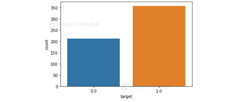
There are a total of 569 data samples and 30 features associated with them. Out of which 212 are malignant samples and 357 are benign.
There are main 10 features in the dataset, and for each the mean, error, or standard error and worst or largest for all these features calculated thus giving us a total of 30 features to work with.
Ten real-valued features which are calculated for each cell nucleus:
- radius (computed as mean distances from center to points on perimeter)
- texture (it is standard deviation of gray-scale values)
- area
- perimeter
- smoothness (variation in radius lengths)
- compactness (perimeter^2 / area – 1.0)
- concavity (severity of concave portions of the contour)
- concave points (total number of concave portions of the contour)
- symmetry
- fractal dimension (“coastline approximation” – 1)
Breast Cancer Project Code
Please download the source code of the breast cancer detection project (which is explained below): Breast Cancer Classification Python Code
Breast Cancer Classification using SVM (Support Vector Machine)
The model we are going to use is the Support Vector Machine for inference on the data. Support vector machine is one of the most commonly used machine learning algorithms. They are used for classification, regression, and also outlier detection. We are going to use it as a binary classification model, which will find a separation boundary from the data that is optimal. It creates the decision boundary by calculating the distance from the closest point for each class called the “maximum margin hyperplane (MMH)”.
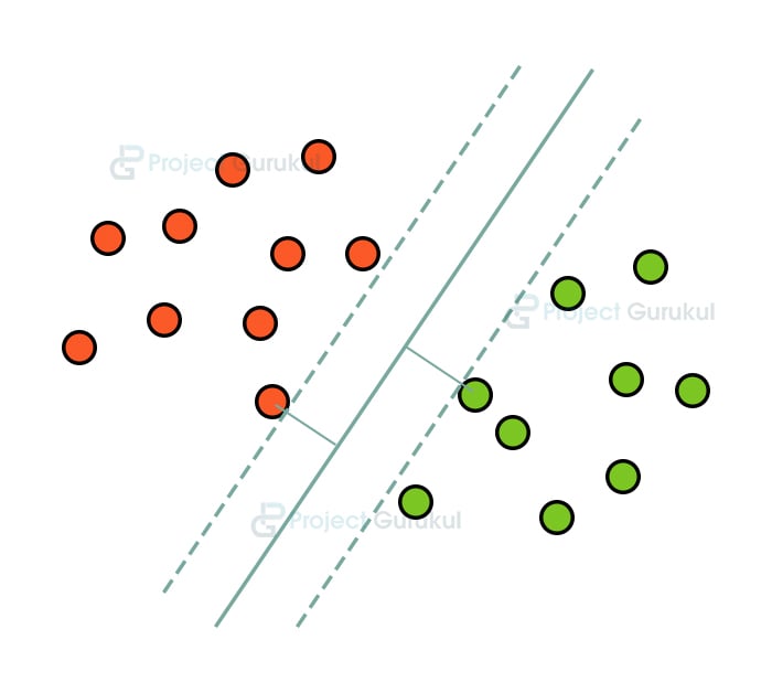
SVM is very useful in high-dimensional spaces. It is highly memory efficient, fast to train and works very well where there is a clear separation margin between the data. It also works well when the number of dimensions exceeds the number of samples.
We will be building the system in Google Colab notebook, which provides a better understanding of data and an easy & simple to use system. You can work in the same way in a jupyter notebook or even in python ide with some changes.
Steps to Develop Breast Cancer Project
1. Import the required libraries
Let’s begin with numpy which helps in working with arrays and data.
Matplotlib to help in visualizing during our exploratory dataset analysis.
Pandas will read the data from the dataset and help in cleaning and arranging the data.
Seaborn will help matplotlib. Using matplotlib inline because we are building the system in a colab notebook.
We are going to use scikit learn or sklearn library for most of the machine learning related tasks. It is one of the most useful and robust machine learning helper libraries in python. It contains lots of helpful tools and also pre implemented models for simple tasks like classification regression and clustering.
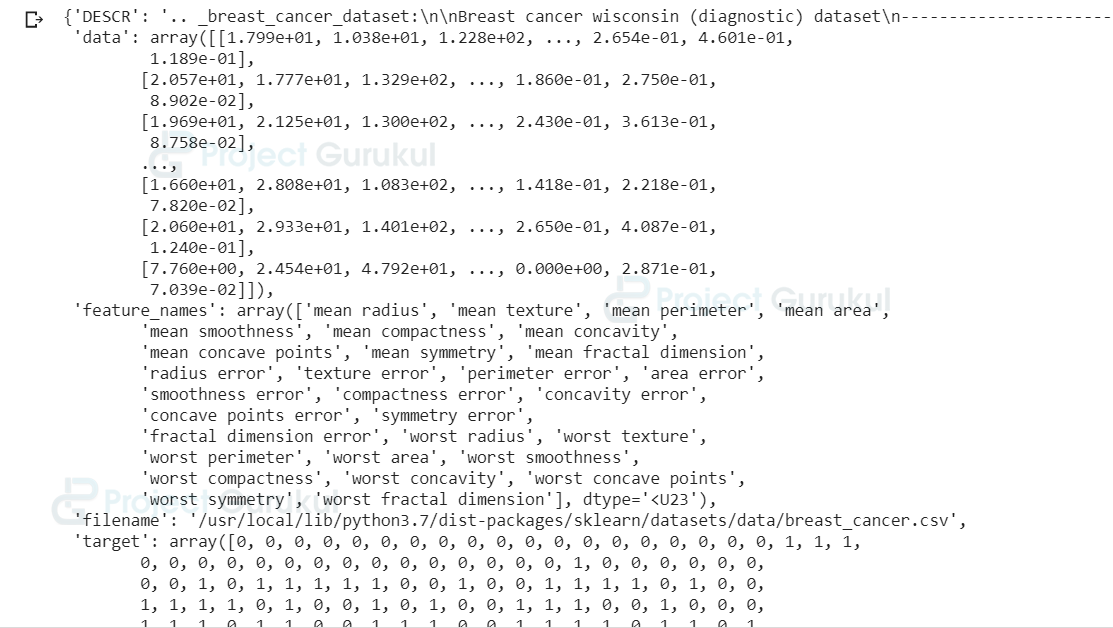
For our task luckily we can directly import the dataset from sklearn but you can also download it from the official UCI machine learning dataset website (link is mentioned in Dataset section).
import numpy as np
import matplotlib.pyplot as plt
import pandas as pd

import seaborn as sns

%matplotlib inline

from sklearn.datasets import load_breast_cancer
Breast_cancer = load_breast_cancer()
This code will print the loaded dataset details in raw format.
2. Data Analysis and Cleaning
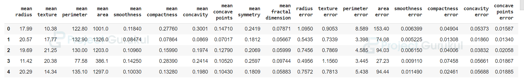
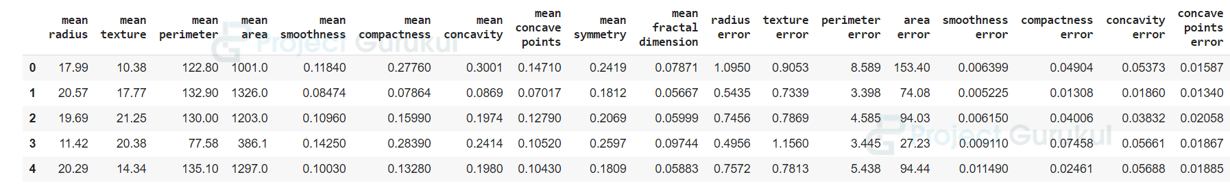
Now we will convert it to a dataframe using pandas to help us understand and work with the data better. Print the first five samples from the dataset using the head function for understanding what the data holds.
Breast_cancer_df = pd.DataFrame(np.c_[Breast_cancer['data'], Breast_cancer['target']], columns = np.append(Breast_cancer['feature_names'], ['target']))

Breast_cancer_df.head()
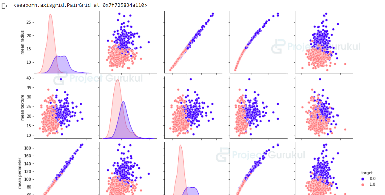
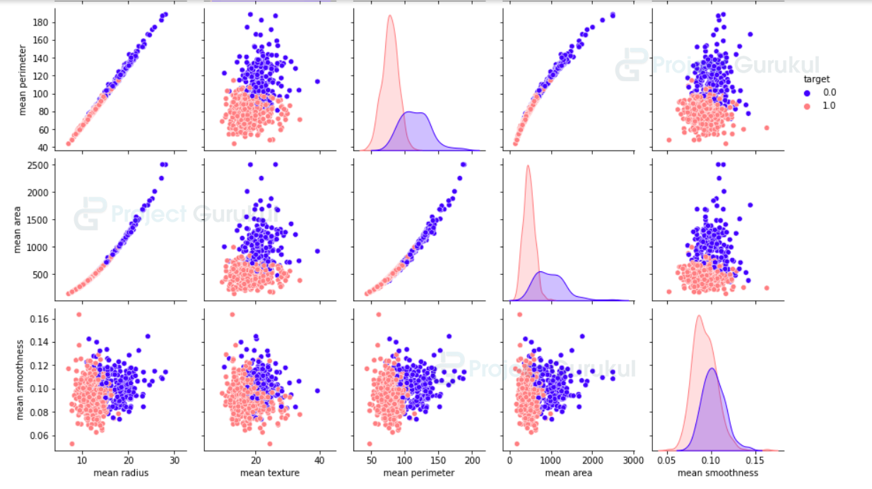
We will print some information about the dataset and then visualize our data. We are going to plot the first five features and also the relationship between them.
Breast_cancer_df.shape
Breast_cancer_df.columns

sns.pairplot(Breast_cancer_df, hue = 'target',palette='gnuplot2', vars = ['mean radius', 'mean texture', 'mean perimeter','mean area','mean smoothness'])
Now we plot a bar graph to visualize the volume of samples we have in each class.
Breast_cancer_df['target'].value_counts()
sns.countplot(Breast_cancer_df['target'], label = "Count")
We get the train data by dropping the target from the dataframe. And then display its head. By just taking the target values we get the target data.
Train_data = Breast_cancer_df.drop(['target'], axis = 1)
Train_data.head()

Target_data = Breast_cancer_df['target']
Target_data.head()
3. Preparing Data for Training
We import the test train split function from the sklearn module and divide the data into test and train parts. Print the details about the numbers of each set.
from sklearn.model_selection import train_test_split
X_train, X_test, y_train, y_test = train_test_split(Train_data, Target_data, test_size = 0.2, random_state = 20)

print ('Number of training samples input is', X_train.shape)
print ('Number of testing samples input is', X_test.shape)
print ('Number of training samples output is', y_train.shape)
print ('Number of testing samples output is', y_test.shape)

We now need to perform feature scaling or normalization on the data so that it is easier for our model to work with it. By scaling the feature values we map it in a certain range mostly 0,1. That is what we are doing here with the training data input and also the test data input.
4. Training the Data
We then import the model from the sklearn library and train it on the data. The fit function takes as input the training data input and the targeted value and trains on it.
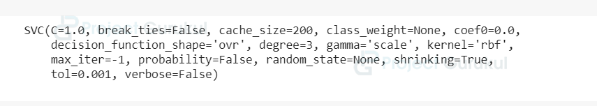
#Feature Scaling
from sklearn.preprocessing import StandardScaler

sc = StandardScaler()
X_train_scaled = sc.fit_transform(X_train)
X_test_scaled = sc.transform(X_test)

#X_train_scaleded.head()

from sklearn.svm import SVC
svc_model = SVC()

svc_model.fit(X_train_scaled, y_train)
5. Getting the Results
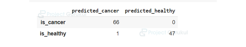
The predictions are the breast cancer classification result of the test data. We pass in the scaled test data input and get the predictions by the model. We then pass the prediction to the confusion matrix along with the target test output to get the confusion matrix.
A confusion matrix has 4 parts:
- True positive: the target was positive the model gave positive
- True negative: the target was negative the model gave negative
- False positive: the target was negative the model gave positive
- False negative : the target was positive the model gave negative
It helps in getting if the model is favoring a certain side.
Prediction = svc_model.predict(X_test_scaled)

from sklearn.metrics import classification_report, confusion_matrix

cm = np.array(confusion_matrix(y_test, Prediction, labels=[1,0]))
confusion = pd.DataFrame(cm, index=['is_cancer', 'is_healthy'], columns=['predicted_cancer','predicted_healthy'])
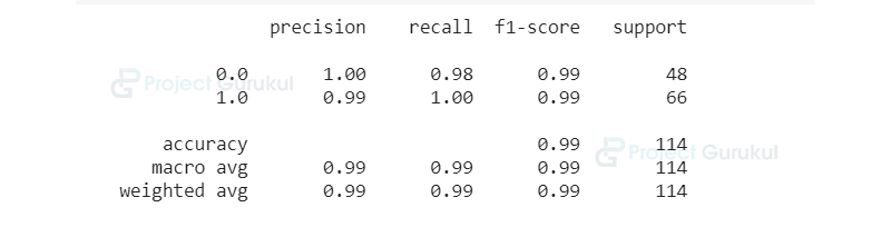
Now we print the precision, accuracy, recall, and f1 scores of the model.
print(classification_report(y_test,Prediction))
Now we have the model we can save it for later use or transfer it to another system by using pickle. We import pickle, create a file with .pkl extension and dupl the serialized data in binary form to that file. In the same way, we open that file and read back that data, then perform predictions or anything that we want.
import pickle

pkl_filename = "pickle_model.pkl"
with open(pkl_filename, 'wb') as file:
    pickle.dump(svc_model, file)

# Load from file
with open(pkl_filename, 'rb') as file:
    pickle_model = pickle.load(file)
Summary
We have successfully built a breast cancer classification system project that is fairly accurate and can help in identifying major kinds of breast cancer.
Early identification and treatment of these diseases can prevent major health hazards and even save lives. The use of computer vision and deep learning has grown extensively in medical examination as an aid to doctors and researchers. There is a shortage of medical experts in our country and we can hope that these systems can reduce the workload and help them in the preliminary stages of examination.